Sim-Diasca Modeller Guide

![]()
![]()
| Organisation: | Copyright (C) 2015-2025 EDF R&D |
|---|---|
| Contact: | olivier (dot) boudeville (at) edf (dot) fr |
| Author: | Olivier Boudeville |
| Creation Date: | March 2015 |
| Lastly updated: | Friday, July 18, 2025 |
| Version: | 2.4.8 |
| Status: | Stable |
| Website: | |
| Dedication: | For people wanting to implement a simulation with the Sim-Diasca engine. |
| Abstract: | We present here the main steps to go through whenever having to create a new simulation with Sim-Diasca, from the definition of the simulation case to the one of the models, the scenarios and any extra simulation service involved. The modelling and the implementation are described on a step-by-step basis, allowing to introduce incidentally the basic features offered by the engine. |
Table of Contents
Note
Before reading this document, we strongly advise to have at least had a first look at:
- the slides of the general-purpose presentation of Sim-Diasca
- the Sim-Diasca Technical Manual, notably its simulation ontology (in chapter 3) and its overall modelling considerations (in chapter 6)
Overview & Context
Objective
Let's suppose we have a simulation to implement. This would be here a simulation in the field of Complex Systems: the system of interest would be described in a disaggregated way, i.e. as autonomous agents whose interactions recreate the overall behaviour and dynamics of that system [1].
| [1] | One can note that not all simulations are naturally described according to such a "complex system" scheme. For example some data-flow computations are typically best described as spreadsheets. However, if it is deemed relevant enough, a simulation engine for complex systems, even if it is certainly not the most relevant tool for that, could be entrust in order to evaluate these spreadsheet-like computations. |
These interactions would be event-based, rather than taking place continuously. For example, they could correspond to an incinerator notifying an operator of a burner failure, to a tramway opening its doors or to a person dialling the phone number of a friend.
Indeed the underlying time is discrete here, and operations last for a duration materialised by punctual state transitions, i.e. events that bear a timestamp in simulation time. If there were quantities that would be continuously changing (like the temperature of a room, depending on the time of the day), their variation would have to be discretised over time first [2].
| [2] | We can see here that models that would be driven mostly by differential equations (over continuous time) are not the primary targets of such simulation engines. Even if a numerical solver could be used underneath and if, in some cases, time could then be safely quantified, correctly mixing discrete-time and continuous-time models in the general case requires a very specific and advanced kind of engine, an hybrid one; only very few engines of this type exist (and, to the best of our knowledge, none is parallel - hence these engines may experience scalability issues). So it seems difficult to rely both on an hybrid mode of operation and on a scalable one. |
So let's see how easy it is to use the Sim-Diasca engine in order to perform such simulations of complex systems, relying for that on a simplified yet representative simulation test case.
Introducing the Engine Thanks to a Step-by-Step Example
We will guide you here through the whole process of creating a brand new simulation of your own, here involving, for the sake of this example, customers trying to obtain soda cans from vending machines in order to relieve their thirst.
Let's name that mock case the Soda-Example simulation case. We will introduce also at its level some stochastic elements to showcase how they should be managed.
We took on purpose a very simple example coming from the everyday life rather than any domain-specific one (e.g. in terms of telecom, or urban planning, or electricity), so that the reader can get familiar here only with the topics directly related to the simulation field, without having them intermingled with additional specific domains.
So, what does creating a simulation always entail?
- defining the simulation case, which is the overall description of the simulation that will rule its actual execution
- defining the "abstractions" of interest in this context, i.e.:
- the models involved, which collectively provide a simplified representation of the target system that is to be simulated
- the scenarios (if any) to account for the context of the target system
- defining the results expected from the simulation, i.e. what are the metrics that shall be collected thanks to probes, and how they should be produced
Let's begin with the overall coordinator, i.e. the simulation case, before discussing more complex subjects with, notably, the models.
Note
This modeller guide concentrates on the Soda-Example test, which we found very useful to demonstrate various aspects of the simulation of complex systems and compare engines.
This case has been fully implemented, and is part of the standard Sim-Diasca distribution, shared as an archived named Sim-Diasca-x.y.z.tar.bz2.
On UNIX (typically GNU/Linux), one should extract it thanks to: tar xvjf Sim-Diasca-x.y.z.tar.bz2. All relative paths mentioned in that document are relative to the root of this extracted archive, i.e. Sim-Diasca-x.y.z.
One can thus refer to the full sources of the Soda-Example test, which are located in mock-simulators/soda-test.
Most of the files of interest lie in its src subdirectory, so, unless specified otherwise, any file that is specific to Soda-Example will be found there. Files that relate to the engine itself are located in the sim-diasca tree of the same archive.
Through this guide, various files will be mentioned - we strongly advise the reader to open them as they are mentioned , since it helps considerably figuring out the general layout, and understanding that there is no magic involved.
Defining the Simulation Case
The purpose of the simulation case is to define all the settings of a virtual experiment that will be run.
This includes defining, for that targeted simulation:
- technical settings, like the properties to be enforced for this simulation (e.g. reproducibility), the time-step to be used or the list of the eligible computing hosts
- domain-specific settings, like the description of the initial state of the simulation (i.e. the model instances that exist when the simulation starts) and its various termination criteria
- experiment settings, like the specification of the results that are expected from the simulation, i.e. what are the probes that shall be enabled, whether these results should displayed to the user, etc.
Multiple experiments may apply to a given simulation (e.g. the Soda-Example one), hence multiple simulation cases are generally devised. For example:
- there could be as many minimalist cases as there would be different models defined (e.g. one case would perform a unit test of the soda vending machine, and each type of thirsty customer would have its own test case as well)
- other simulation cases could serve to test the interactions between such a machine and a given type of customer
- finally overall integrated cases could exist to provide the actual targeted simulation(s), with their final settings, scale, bells and whistles
Where Shall a Simulation Case be Defined?
All the information relative to a simulation case are to be specified into a single file, named according to that simulation case.
If we were to define a test that would focus on the loading of initial instances for our Soda-Example, then we could name the corresponding simulation case soda_loading_test and implement it in a text file named soda_loading_test.erl.
The .erl file extension corresponds to Erlang source files, knowing that Sim-Diasca uses this programming language for its implementation (one may refer to Just A Bit of Computer Science To Better Understand The Whole for more information on that topic).
Now is the right time to have soda_loading_test.erl [3] opened in your favorite text editor (e.g. Emacs, Eclipse, etc. - preferably with a support for the highlighting of the Erlang syntax).
| [3] | As mentioned earlier, this file is located in the Sim-diasca-x.y.z/mock-simulators/soda-test/src directory. |
The Three Main Settings Records
Most of the elements mentioned in a simulation case are to be specified in predefined records, which are Erlang data-structures (say, to describe a person) containing named fields (for example to store information about that person, like his name, phone, address, etc.).
Three records play a central role in simulation cases and will have to be specified in order to initialise the engine:
- the simulation_settings record, gathering information about the simulation itself (name, tick duration, etc.)
- the deployment_settings record, gathering information about its context of deployment and execution, knowing that Sim-Diasca is a distributed engine (e.g. computing hosts potentially involved, extra elements to deploy, extra services to activate)
- the load_balancing_settings record, gathering information about how the computing resources shall be allocated to the various parts of the simulation
Sensible default values are defined for most of the fields of these records. In this modeller guide, we will mainly discuss the ones that should be overridden for this example [4].
| [4] | For a complete description of these three records, please refer to the Sim-Diasca Technical Guide or directly to their definition, respectively in the following header files in the sim-diasca tree: class_TimeManager.hrl, class_DeploymentManager.hrl and class_LoadBalancer.hrl (the .hrl extension denotes Erlang header files). |
Simulation Settings
Let's discuss first the technical parameters that shall be specified in various fields of the simulation_settings record that you can find in soda_loading_test.erl.
For the sake of clarity, a simulation should preferably have a name of its own - to be defined in the simulation_name field. An adequate naming is convenient to discriminate more easily among runs and result sets [5].
| [5] | Both of them benefit from mechanisms that prevent any two simulation runs to step on each other. Names are here only to help humans! |
Let's forfeit any creativity and name our case "Sim-Diasca Initial State Loading Test".
We must also define the duration (in virtual time) of the fundamental time step of the simulation (or its evaluation frequency), i.e. its overall tick duration. This is probably the most important setting for synchronous simulations - to be defined in the tick_duration field, as a floating-point number of seconds.
This corresponds to the finest granularity of time that the simulation will be able to discriminate. This may relate also to how reactive the simulated world must be.
The models involved in a simulation have a temporality of their own (a model is not even aware of the various simulation cases that may include it) and will rely only on high level, absolute durations (in virtual time of course), expressed for example as "2 hours" rather than as a number of ticks.
As a result, models are defined regardless of the actual frequency at which simulations incorporating them will be run, i.e. irrespective of the tick duration chosen by each simulation case. This offers much flexibility to the simulations, and removes one cause of interdependence between models.
Of course an infinite leeway cannot be granted: ultimately, at runtime, these models will have to convert the high level durations they embed (e.g. 2 hours) into a (positive) integer number of ticks, and of course the overall tick duration of the case must be fine enough in order that this quantification does not introduce too much inaccuracy [6].
| [6] | To anticipate a bit, the Actor class provides relevant primitives for that, including convert_seconds_to_ticks/2; should, at execution time, the conversion lead to a relative error greater than the default threshold, the simulation will be stopped on error. convert_seconds_to_ticks/3 allows the modeller to specify his own threshold, on a per-conversion basis. |
So, why not defining in the simulation case a very small evaluation period (tick duration), to ensure that, for all models, their embedded high-level durations will be nicely mapped to ticks?
Well, this is certainly possible, yet generally it forces the engine to schedule more ticks, resulting in a decrease of the performances of the simulation. Yet Sim-Diasca offers a relatively advanced scheduling (notably able to determine ticks that have no impact and jumping over them), which may mitigate that problem.
Anyway a reasonable trade-off must be found, and in this test case we opt for a rather fine granularity, namely a simulation frequency of 100Hz, i.e. a tick duration of 0.01 second. Most simulations will elect far longer time-steps, some of them for example opting for a yearly basis. This depends much on the application domain.
Another information to specify in the simulation_settings record is the results we want to obtain from the simulation. Here we will go for the simplest solution, using the default value of the result_specification field, which is to retain all outputs. Other settings allow to filter results by probe type, or based on a series of targeted and blacklisted patterns applied to the names of the potential results [7].
| [7] | Please refer to the section 11.2 of the Sim-Diasca Technical Manual for more information, or directly to the documentation of the result_specification field in the class_TimeManager.hrl header. |
So, finally, our simulation settings (that we store here in a variable that we name, for clarity, SimulationSettings - in Erlang, variable names start with a capital letter) can then simply be defined as:
SimulationSettings = #simulation_settings{
  simulation_name="Sim-Diasca Initial State Loading Test",
  tick_duration=0.01
}
As mentioned, two other records aggregate the rest of the technical settings.
Deployment Settings
The deployment_settings record allows to set precisely the computing hosts involved in the execution of that simulation case.
Sim-Diasca can indeed run a simulation on the user host only (the computer on which it is run), yet it is a distributed engine - so a single simulation can be also run on a set of computers (potentially dozens of nodes of a high-performance computing cluster).
For our simulation case to be able to run indifferently either on a single host or on multiple ones, the computing_hosts field will be set to request the engine to check first whether a text file, named here sim-diasca-host-candidates.etf, can be found. The purpose of this file is to list the host names of all the potential computers that may be involved in the simulation [8].
| [8] | Please refer to the section 19.2 of the Sim-Diasca Technical Manual for its actual syntax (hostnames but also per-host usernames can be specified), or look directly to sim-diasca-host-candidates-sample.etf, to be found in the sim-diasca/conf directory. |
If this host file is found, the engine will look-up and try to use as many of the host candidates listed there as possible (depending on their availability and on the checking of various prerequisites).
If this host file is not found, or if it does not list any usable host, the case will run only locally, on the user computer.
So the definition for this field of the deployment_settings record boils down to:
computing_hosts = {use_host_file_otherwise_local,
                   "sim-diasca-host-candidates.etf"}
That same deployment_settings record is also the place where we can define the simulation elements (code and data) beyond the mere engine that shall be deployed on the computing nodes. This includes typically the binary files corresponding to the implementation of the models and scenarios [9], possibly with any set of data files they might rely upon.
| [9] | In a similar way as Java, Erlang sources (*.erl files), possibly with their headers (*.hrl), are compiled into bytecodes (*.beam files) that are to be executed by a virtual machine (the Erlang VM). So Sim-Diasca starts one virtual machine per computing host (that will federate all its CPUs and all their cores) and sends over the network a compressed archive containing notably the relevant BEAM files to each of these virtual machines. |
Our Soda-Example case involves only a few models (e.g. model of the soda vending machine, or of a type of customer) - that will be defined in the same directory as this simulation case - and no specific data, thus setting the following field accordingly will be sufficient:
additional_elements_to_deploy = [ { ".",code} ]
This means select all code (BEAM files) recursively found from the current directory (".", i.e. mock-simulators/soda-test/src here) and add it to the deployment archive.
Still in the deployment_settings record, other parameters can be set (e.g. node_availability_tolerance) and other services can be activated (e.g. enable_data_exchanger, enable_performance_tracker), yet the Soda-Example case can do without them. So for this record, which we choose to store in a variable named DeploymentSettings, we finally end up with the following definition:
DeploymentSettings = #deployment_settings{
    computing_hosts = {use_host_file_otherwise_local,
                       "sim-diasca-host-candidates.etf"},
    additional_elements_to_deploy = [ {".",code} ]
}
Again: long to explain, very short to specify!
Load Balancing Settings
As there is no specific measure to be taken regarding load balancing here, the corresponding record will be used with all its default values set (no field specifically overridden).
We name our variable consistently with the two previous ones, for clarity, so we have:
LoadBalancingSettings = #load_balancing_settings{}
As a result we now have determined the three key records (regarding simulation, deployment and load balancing) that will allow to initialise the engine. That will be done simply thanks to:
DeploymentManagerPid = sim_diasca:init(SimulationSettings,
           DeploymentSettings,LoadBalancingSettings)
This shall be read as:
- we have a module named sim_diasca
- which exports a function named init
- that takes three parameters (our three records)
- and returns a value, stored in a variable that we named DeploymentManagerPid
We say that the arity (number of parameters) of this function is 3, and that its full name is sim_diasca:init/3.
The returned value is a PID, an Erlang shorthand for process identifier. Knowing the PID of a process allows to send messages to it; here we will then be able to send messages to the deployment manager of the engine, from the simulation case.
In Erlang, one can optionally specify the signature of a function, i.e. the types of its parameters and of its returned value.
Such a type specification clarifies the code and the developer's intent, and allows some static type checking tools to perform more in-depth verifications.
Here this would be a pretty self-explanatory specification [10]:
-spec sim_diasca:init(simulation_settings(),deployment_settings(),
              load_balancing_settings()) -> pid().
| [10] | One may refer to Types and Function Specifications for more information. -spec is to be used for functions, while -type is to be used for terms (i.e., values). For example, -type age() :: integer(). tells that a variable of type age is an integer. |
Let's continue now the simulation specification by its heart: the models.
Defining the Models
General Outline
Here we will focus on a Soda-Example simulation in which there would be:
- two kinds of thirsty customers, whose repletion duration [11] obey different rules
- a single sort of soda vending machine, selling a single sort of soda
| [11] | Defined as the duration after which their thirst reappears once having been extinguished (i.e. once having drunk a soda can). |
Hence we have here three different models. All other elements (the outside world, the floor, the room, the other persons, the electric supply, the cans themselves, etc.) are considered as irrelevant for this study, and thus are abstracted out (i.e. they will not be represented explicitly in the simulation, short of influencing it).
Of course, for a given model (which can be seen as a description of a type, i.e. an abstract blueprint), any number of actual instances may exist, each with its own, individual state and fate. A shorthand for model instance that will be used from now is actor.
As always, several instances of these models (i.e. several simulation actors) must be able to interact gracefully with respect to the simulation expected properties in order to produce its expected outcome, i.e. the simulation results that were requested by the user.
For this simulation we consider that the results that we are interested in are the stock of cans that each vending machine holds over time.
We thus want to obtain from the simulation a time series for each machine stock (as a data file), and its corresponding plot (as an image). Both of them will be produced by probes (one probe per vending machine).
As there is no refill of the machines modelled, we would expect the stocks to steadily decrease over simulation time.
Let's ensure first that we will be able to create the model instances we need.
Construction Parameters
Having a simulation requires to define, among other elements, its initial situation, i.e. what are the model instances that exist when the simulation is to begin.
To do so, we need to be able to define, for each model, how many instances must exist from the start [12], and in which state they are initially.
| [12] | Any simulation must have at least one initial actor. Of course, in the general case, actors may also be created (and deleted) in the course of the simulation. |
For that, a model has to define at least one constructor, which is a function (named construct) that translates a set of construction parameters into an actual instance of this model, created from them [13].
| [13] | Constructors are essential to preserve encapsulation, i.e. to ensure that the inner implementation of a model remains private to this model. Indeed, if, instead of relying on a constructor, the initial state of an actor could be directly set from outside, then the code creating instances of a model would have to know how the state of this model is structured. As a result, that code would depend on the implementation of this model, and a change in the model would propagate to the code using it. On the contrary, constructors allow for a better uncoupling: should the model implementation be updated (then probably impacting how its state is defined), it may require only a change in how its constructor is implemented (construction parameters being then translated differently) - while the interface of that constructor would not change, and then would not impact the code outside of this model. |
Construction Parameters for a Soda Vending Machine
We will suppose here that a given soda vending machine instance can be created from following construction parameters:
- its name, as a character string (e.g. "My soda machine") [14] - a type designated as string()
- the number of soda cans it stores initially, as a positive integer (e.g. 100), of type can_count() [15]
- the unitary cost of the soda cans that it sells, as a floating-point cost in euro (e.g. 1.2 euro per can), of type amount() [16]
| [14] | Naming instances is useful to help understanding the results and the simulation traces that they may produce. |
| [15] | Defined in this case as -type can_count() :: basic_utils:count()., i.e. a positive integer. |
| [16] | Defined in this case as -type amount() :: float()., i.e. a floating-point number. |
These three construction parameters will be enough to create any instance of vending machine. Note that we have no idea yet of how the state of a vending machine will be structured - that is the point of using construction parameters.
Construction Parameters for a Thirsty Customer
As for customers, we mentioned that in our simulation there were two kinds of them; indeed we consider that there are:
- "deterministic" customers, which are thirsty again after a constant duration (e.g. 15 minutes after having drunk)
- "stochastic" customers, whose repletion duration is determined by a random law in order to illustrate their use (e.g. the duration will be drawn from an exponential law of rate parameter lambda=2.2)
So a deterministic thirsty customer instance can be defined from following construction parameters:
- his name, as a character string (e.g. "John") - a string()
- the vending machine he knows, as an instance reference [17] - a type designated as class_Actor:actor_pid(), which is actually an alias for pid(); we see here that we consider that such a customer knows exactly one vending machine - neither none, nor multiple ones (we would have defined in this case a list of PIDs)
- his repletion duration, i.e. how soon, after having drunk a soda can, he will feel thirsty again (e.g. exactly 2 minutes - he is deterministic), of type duration() [18]
- his budget, i.e. how much money he initially has in his pocket (e.g. 35.0 euros) - of type amount()
| [17] | An instance must know another instance ("have a reference onto it") in order to interact with it ("send a message to it"). Technically, a reference onto another model instance is named here an Actor PID, or PID (shorthand for Process Identifier, of type pid()). Actually we have -type class_Actor:actor_pid() :: pid(). |
| [18] | Defined in this case as -type duration() :: unit_utils:minutes(). |
So a deterministic thirsty customer will require these four parameters in order to be created.
Finally, a stochastic thirsty customer will be constructed quite similarly, except that its repletion duration will not be specified as a constant, but as a random law. For example his repletion duration in minutes could be drawn from a Gaussian law whose mean is 10, and variance is 2.
Its constructor shall thus reflect this: the repletion duration that had to be set for the deterministic customer is replaced, in the construction parameters of the stochastic one, by a random law, of type class_RandomManager:random_law() [19].
| [19] | Defined in class_RandomManager.erl. |
From Construction Parameters To Constructors
Now that we have specified the construction parameters that will be used, we will have to define in later steps how the state of these models will be stored.
Then only we will be able to define their constructors, which are the functions that convert the former (the construction parameters) into the latter (the initial state of the corresponding models).
But, for that, the implementation must be better known: the structure of the state of the model will have to be determined first.
Implementation Files
Just A Bit of Computer Science To Better Understand The Whole
Erlang
Sim-Diasca is developed in the Erlang programming language. This functional and concurrent language is a very good fit for problems that can be solved thanks to a (possibly large) number of autonomous logical processes running in a parallel and, possibly, distributed way (i.e. respectively able to take advantage of multiple core and processors, and of multiple networked computers).
Note
Have no fear, though: using Sim-Diasca does not require any knowledge about parallelism, as it is fully hidden by the engine, and models are to be written in a simple, fully sequential setting.
So the purpose of these more technical explanations is only to give to the modellers a better view of the mechanisms involved underneath, as dealing with black boxes may be uncomfortable.
In a few words, an Erlang program is made of several (Erlang) processes that run concurrently and that communicate between them solely through the sending of asynchronous (non-blocking) messages.
WOOPER
Erlang thus provides an excellent multi-agent platform, on top of which we added a thin layer named WOOPER, which provides the language with object-oriented capabilities: WOOPER allows to define classes that can inherit from others (e.g. the Cat class is a specialisation of the Animal class), whose state is defined thanks to a set of attributes (e.g. a cat may have an age attribute, of type positive integer, and a name attribute, of type string), and that can define methods (i.e. class-specific, parametrised signals that a class instance can receive and that will trigger operations based on its state ; e.g. getAge/1, meow/1, declareBirthday/2).
Sim-Diasca
Sim-Diasca has then been added on top of WOOPER, turning a concurrent, object-oriented multi-agent platform into a simulation engine for complex systems: the general simulation infrastructure has been defined (e.g. simulation cases, models, scenarios, probes), and key services have been implemented (like scheduling, interaction support, instance life cycle, loading of the initial state, trace management, result management, deployment, load-balancing).
The engine takes care of the full technical plumbing needed (e.g. proper reordering of the actor messages so that simulation properties are respected), hence Sim-Diasca users just have to comply with the engine's conventions and define their domain-specific simulation elements.
As a result, models can be defined based on a very small, simple subset of the Erlang language. Each model will be a child class [20] of the class_Actor abstract class. Typically each model will define the attributes that make up for its state, the actor methods it supports, and at least one constructor. Of course a given model can inherit from another, allowing for a flexible model hierarchy.
| [20] | Be it a direct child class or not: indeed a model may inherit from other model(s) that will themselves inherit, ultimately, of class_Actor. |
These models will then be able to take part to the simulations of interest.
In Practice For Our Soda-Example Case
As we have seen, three models will be needed. They will thus be implemented in three corresponding classes:
- the SodaVendingMachine model will be implemented as class_SodaVendingMachine, specified in the class_SodaVendingMachine.erl file
- the DeterministicThirstyCustomer model will similarly be implemented in the class_DeterministicThirstyCustomer.erl file
- and of course the StochasticThirstyCustomer model will be in the class_StochasticThirstyCustomer.erl file
(as mentioned, all these files are to be found in the mock-simulators/soda-test/src directory)
The class_ prefix is mandatory to specify that we are defining a WOOPER class (and not a basic Erlang module), and, as mentioned previously, the .erl file extension corresponds to Erlang source files (i.e. that contains the Erlang code corresponding to the module of the same name).
We can see that each model will be defined separately from the others, and that it will be contained in a single, standalone source file.
For the sake of this simple test case, none of these models will inherit from others: all three will be direct child classes of the class_Actor abstract class.
A slightly more complex alternative would have been to define an abstract ThirstyCustomer model directly deriving from Actor, from which DeterministicThirstyCustomer and StochasticThirstyCustomer would have then derived.
As we can see, there are often multiple ways of modelling the same target system. We chose the simplest here.
Initial State of the Simulation
Of course an engine cannot guess what the initial content of the simulation will be (it will simply start from it, and make it evolve until reaching a termination criterion), so we have somehow to specify the initial simulation state. This information is to be specified in the simulation case.
Two methods are available for that: either we create initial instances thanks to code, or thanks to data.
Creating Initial Instances Programmatically
For this test case, we want following basic initial setting to be simulated:
- there will two soda vending machines (referenced as SVM1 and SVM2)
- there will three thirsty customers: TC1 and TC2, who will be both using SVM1, and TC3, who will use SVM2; TC1 and TC3 shall be deterministic customers, while TC2 will be a stochastic one
This corresponds to the following setting:
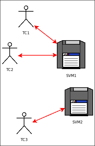
This is a fairly simple simulation, where no actor is created or deleted in its course. So it will begin and end with exactly the same five model instances (but f course their respective state will change over the simulation).
These instances will be created programatically in this example: the simulation case will explicitly create them, by code, one by one.
Actually, even if the implementation of the models is not known yet, we can already determine the corresponding snippet that will be part of the simulation case in order to create the expected initial instances.
We must just know that:
- initial instances must be created by using the class_Actor:create_initial_actor/2 static method, whose first parameter is the name of the class of the instance to create (e.g. class_Incinerator), and whose second one is the (ordered) list of the construction parameters for that upcoming instance
- in Erlang:
- comments start with the % character
- as mentioned, a variable name starts with a capital letter (e.g. MyVariable) but prefixing it by an underscore (e.g. _MyVariable) makes it a mute variable, i.e. a variable that will be ignored by the compiler - so specifying it just serves documentation purposes
- a list is denoted by brackets, and may not be homogeneous (e.g. MyList=["hello",42])
These programmatic creations translate as:
% First machine starts with 100 cans, 2 euros each:
SVM1 = class_Actor:create_initial_actor( class_SodaVendingMachine,
    [ _FirstMachineName="First soda machine", _FirstInitialCanCount=100,
      _FirstCanCost=1.0 ] ),

% Second machine starts with 8 cans, 1.15 euro each:
SVM2 = class_Actor:create_initial_placed_actor( class_SodaVendingMachine,
    [ _SecondMachineName="Second soda machine", _SecondInitialCanCount=8,
      _SecondCanCost=1.15 ], _PlacementHint=gimme_some_shelter ),

% First customer is deterministic, uses SVM1, is thirsty 2 minutes
% after having drunk, and has 35 euros in his pockets:
_TC1 = class_Actor:create_initial_actor(
  class_DeterministicThirstyCustomer,
  [ _FirstCustomerName="John", _FirstKnownMachine=SVM1,
    _FirstRepletionDuration=2, _FirstInitialBudget=35.0 ] ),

% Second customer uses SVM1 too, yet is stochastic: he will be thirsty
% again between 1 and 7 minutes after having drunk, and has 40 euros in
% his pockets initially:
_TC2 = class_Actor:create_initial_actor( class_StochasticThirstyCustomer,
  [ _SecondCustomerName="Terry", _SecondKnownMachine=SVM1,
    _SecondRepletionLaw={ uniform, 7 }, _SecondInitialBudget=40.0 ] ),

% Third customer uses SVM2, is deterministic and thirsty 2 minutes
% after having drunk, and has 77 euros in his pockets:
_TC3 = class_Actor:create_initial_actor(
  class_DeterministicThirstyCustomer,
  [ _ThirdCustomerName="Michael", _ThirdKnownMachine=SVM2,
    _ThirdRepletionDuration=2, _ThirdInitialBudget=77.0 ] ),
Scrupulous readers noticed that the creation of SVM2 actually relies on a variation of class_Actor:create_initial_actor/2.
This static method, named class_Actor:create_initial_placed_actor/3, takes an extra parameter: a placement hint. The engine will ensure that all instances created with the same hint (here, the gimme_some_shelter atom [21]) will be co-allocated, i.e. created on the same computing node (whichever it is).
This allows to deliver locally the numerous messages they exchange, which is a lot more efficient than sending them through a network.
Thus a user knowing that by design a set of instances will be tightly coupled (for example, models of a modern human being and of his beloved smartphone) is able to have them co-allocated for best performances, irrespective of how the simulation case, depending on each simulation run, will be later dispatched on a set of networked computing nodes.
Here, at least another initial instance should be created with gimme_some_shelter for this hint to be useful.
| [21] | An atom is an Erlang datatype that allows to define a symbolic constant. Typically an atom begins with a lower-case letter (as opposed to variables). For example hello and class_Cat are atoms. |
Creating Initial Instances From a Data Stream
Of course "real" simulations tend to be far more demanding than the previous case relying on five actors, and may involve literally millions of model instances.
It would be unlikely that such a large number of actors be created programmatically; instead these actors should preferably be instantiated from a data stream, typically a text file.
Sim-Diasca provides a simple, compact, flexible format to do so; as always, initial creations are to be triggered from the simulation case.
In a few words, remembering that the construction parameters of a soda-vending machine are [MachineName,InitialCanCount,CanCost], creating such a machine would just boil down to having, in said data file, a line like:
{ class_SodaVendingMachine, ["Machine #1 read from data",
                              45,1.5] }.
If wanting to be able, in another point of the data stream, to refer to an initial instance, then its creation shall be prefixed by the specification of a user identifier ("My second machine" here), like in:
"My second machine" <- { class_SodaVendingMachine,
                            ["Machine #2",4,1.4] }.
Then other initial instances could refer to that instance (i.e. know it at construction time), like in:
{ class_DeterministicThirstyCustomer, [ "Cresus",
  {user_id,"My second machine"}, 12, 16000.0 ] }.
Here, remembering that the construction parameters of a deterministic thirsty customer are [CustomerName,KnownMachinePid,RepletionDuration,InitialBudget], the customer named Cresus would detain a reference (translated into a PID at construction time) onto the vending machine named Machine #2.
As a result, the customer will be able to interact with the machine from the simulation start (since it will know the PID of this machine). Until it has done so (thus letting the machine knows about its own PID), the machine will not be aware of him (as here, by design, it has no means of knowing that customer).
In such an initialisation data stream, the order of the lines does not matter, cyclic references are supported (so we could define two actors mutually aware of the other), and comments (lines starting with %) and blank lines are ignored.
One may refer to the soda-instances.init data file as a full example.
For a simulation case to read initial instances from such an initialisation file, the corresponding filename must be listed in the initialisation_files field of the simulation_settings record, like in:
[...]
SimulationSettings = #simulation_settings{
  [...]
  initialisation_files = ["soda-instances.init"]
  [...]
},
[...]
One may refer to the section 10.3 of the Sim-Diasca Technical Manual for more information about instance creation.
What About Scenarios?
Instance creation has been discussed, and we saw how actors (model instances) shall be created.
As mentioned in our mini-ontology about simulation (see chapter 3 of the Sim-Diasca Technical Manual), the overall simulated world is the union of the target system and of its context.
While the target system as a whole (e.g. a city) is described based on the various models involved (e.g. buildings, roads, people), in a simulation this target system might have to be evaluated on par with a context that may interact with it (e.g. the country surrounding that city, the weather system over its districts, the mayor and his team).
How shall this context be described, initialised and evaluated then? The good news is that if, semantically, the target system and its context are different, technically they have to be managed the same, notably to preserve simulation properties.
Knowing that the context is made of scenarios exactly like the target system is made of models, creating the context (which, in the general case, can be disaggregated, can have a state, can interact with its parts and with the target system) is to be done exactly as shown previously with the models.
So multiple scenarios may apply (e.g. regarding weather, pollution, population) and multiple instances of them can coexist concurrently (e.g. one weather cell per spatial subdivision of the city).
For example, like we defined class_SodaVendingMachine we could define class_CanCostScenario, an horrible scenario that would reproduce a creeping inflation and would make the price of soda cans steadily increase over time.
An instance of such scenario would be created from two construction parameters, the (supposedly constant) monthly cost increase (e.g. 7%, hence 0.07) and the list of the soda vending machines that would be affected by this inflation.
Then, taking a programmatic creation as an example, we could have:
_SC = class_Actor:create_initial_actor( class_CanCostScenario,
    [ _MonthlyRate=0.07, _VendingMachines=[SVM1,SVM37] ] )
We can thus see that nothing more than models is to be learned in order to manage scenarios, since they are technically the same beast. As hinted by the static method used here, which is defined in the context of the Actor class, the engine does not even make a difference between models and scenarios.
Note
Implementing such a CanCostScenario scenario is left as an exercise for the reader.
This would include going through the same steps as for the models that we will implement here (defining state, behaviour, etc.), notably defining the interactions between a cost scenario and the vending machines that it drives.
For example, the specification could dictate that each month the scenario would notify each machine it knows that its can cost increased, here, of 7%, compared to the previous month.
Instanciation Example
Of course the two approaches (programmatic/data-based) for instance creation can be mixed. One may refer to our simulation case of interest here (soda_loading_test.erl) that creates 5 initial actors thanks to code, and 9 others thanks to the soda-instances.init data file it refers to (in its initialisation_files field).
So we started the work on the models by establishing their construction parameters, in order that the initial state of the simulation could be defined, in the simulation case.
As now this case is almost complete, let's discuss the last few bits necessary to the implementation of a case, before continuing the work on the models.
Wrapping-Up the Simulation Case
Now the engine is correctly initialised (thanks to the three aforementioned settings) and the initial state is defined. What remains to be specified then?
Initial Time and Date
By default, a simulation starts on the first of January of year 2000, at 00:00:00. The Soda-Example relies on that default, but some cases will want to override that.
The initial simulation timestamp can be changed by communicating a new date and time to the root time manager [22] (from the simulation case and, obviously, before the simulation is started).
First step is to retrieve a reference (a PID) onto this root time manager. It can be obtained thanks to the PID of the deployment manager, which is the entry point of the simulation that was returned by the call to sim_diasca:init/3 that we already mentioned:
[...]
DeploymentManagerPid = sim_diasca:init(SimulationSettings,
            DeploymentSettings,LoadBalancingSettings),
[...]
DeploymentManagerPid ! {getRootTimeManager,[],self()},
| [22] | The root manager is the one in charge of the overall scheduling of the simulation: in a purely local setting (a single node), there is only one time manager, while in distributed mode there is one local time manager per computing host, all of which synchronising themselves with the root one. In a more general view, a scheduling tree of time managers, potentially of arbitrary depth and shape, may exist. |
Explaining this last line is a good occasion to introduce more information about how Erlang is to be used.
Erlang processes communicate between them solely thanks to the sending of messages. This sending is asynchronous: a process A having to send a message M (whatever it is) to a process B (designated by its PID, stored in the BPid variable) will simply have to specify: BPid ! M.
As mentioned, all Erlang processes live concurrently, i.e. they are all executed in parallel. Unless a process is looping over its code or blocked in a receive clause (waiting for a message to be received), it will simply terminate.
This message (M) can be any Erlang term, for example the content of any Erlang variable. Here, in our simulation case, the message that we saw is a tuple (i.e. a fixed-length series of terms) of three elements [23] (respectively here: the getRootTimeManager atom, the empty list [] and the result of a call to the self/0 function). This last function returns the PID of the current process, namely here the one executing currently the simulation case.
| [23] | A tuple of three elements ({X,Y,Z}) is named a triplet. A tuple of two elements ({X,Y}) is named a pair. |
A message is sent in a "fire and forget" manner: the sending process, A, will transfer it to the Erlang runtime and directly continue with its next instructions, without waiting for example that B receives it [24].
| [24] | Once actually received (either locally or transparently through the network) this message will be stored in the mailbox of B, which will be free to read it whenever it deems it appropriate. Note that only the message itself (M) is delivered; as a result, by default B has no means of determining what process sent it. If B needs this information, then A may send for example the term {M,APid} instead (and of course B shall expect to receive such a pair). |
When the simulation case sends the {getRootTimeManager,[],self()} message to the deployment manager, this Erlang message will be interpreted according to the WOOPER conventions: the getRootTimeManager request method (i.e. a method returning a result, as opposed to oneway methods that do not return anything) of the deployment manager will be executed (here with no specific parameter, since the specified list is empty) and its result (here, the PID of the root time manager) will be returned to the sender (here, the simulation case, which specified its own PID for that, as last element of the triplet).
As a result, the PID of the (root) time manager will be returned by the deployment manager and stored in the RootTimeManagerPid variable thanks to:
RootTimeManagerPid = test_receive()
So now the simulation case knows the PID of the root time manager, and is able to interact with it.
This allows us to finally specify the initial simulation timestamp discussed in this section, simply thanks to:
% Let's start on 2020, October 21st at 7h, 12 minutes
% and 10 seconds:
StartYear = 2020,

StartDate = {StartYear,10,21},
StartTime = {7,12,10},

RootTimeManagerPid ! {setInitialSimulationDate,
                         [StartDate,StartTime]}
So here we called the setInitialSimulationDate oneway method (we do not expect any result when setting a date) of the root time manager to have its initial simulation timestamp set.
Termination Criteria
The engine must of course have also some way of determining when the evaluation of the simulation shall be stopped.
Multiple criteria can be defined, the first that applies will be the one to actually end the simulation.
Typically the models and scenarios may decide of the termination (e.g. "stop when we reach this total cost or this level of pollution", or "stop when its combination of events happens").
The simulation case can also define such a criterion, typically to mark an upper bound to the duration of the simulation.
Supposing we defined the initial time and date as described in the previous section, we can now define also its maximum duration, i.e. conversely define the final simulation time and date. This could be done thanks:
% We will end exactly 5 years later:
SimulationDurationInYears = 5,

EndDate = {StartYear+SimulationDurationInYears,10,21},
EndTime = StartTime,

RootTimeManagerPid ! {setFinalSimulationDate,
                           [EndDate,EndTime]}
So here the simulation will end no later (as other termination criteria may be triggered first) than the 21st of October of year 2005, at 7h, 12 minutes and 10 seconds.
Starting the Simulation
The simulation can be started simply by requesting the root time manager to do so:
RootTimeManagerPid ! start
This message will therefore trigger the start/1 oneway method of the root time manager.
By the way, one may wonder why this call (i.e. the message sending) visibly does not involve any parameter (e.g. we have BPid ! myMethod, not BPid ! {myMethod,["hello",42]}) yet triggers start/1 (whereas we could expect it would trigger start/0).
The reason is that the Erlang process corresponding to a WOOPER instance keeps internally the state of this instance in a term (of type wooper:state() [25]), and that this state is added as first argument when calling a method.
| [25] | A wooper:state() variable is actually an associative table whose keys are the names of the attributes of the instances, and whose values are the corresponding values (e.g. like a dictionary in Python). For example, if a cat instance is defined by his name and fur color, a cat state could comprise two name/value attribute pairs, such as {name,"Felix"} and {fur_color,black}. |
So, typically, here the message sending would trigger class_TimeManager:start/1 that way:
-spec start(wooper:state()) -> oneway_return().
start(State) ->
  % Actual implementation of that method.
  [...]
We can see first the type specification for this Erlang function (such a specification is optional, yet we recommend writing it down, in order to rely on clearer code that moreover can be more thoroughly type-checked).
The function is named start, takes one parameter (the state that WOOPER keeps and adds automatically) and returns as a oneway (meaning that it only returns an updated state, kept by WOOPER, and no specific result).
The Soda-Example case uses a variation of this start oneway, defined as class_TimeManager:startFor/3 and that can be called with:
% In (virtual) seconds:
SimulationDuration = 150,
RootTimeManagerPid ! {startFor,[SimulationDuration,self()]}
The corresponding definition is:
-spec startFor(wooper:state(),unit_utils:any_seconds(),pid())
    -> oneway_return().
startFor(State,Duration,SimulationListenerPID) ->
  % Actual implementation of that method.
  [...]
Here, beside the usual state, the oneway specifies a duration (the maximum one for the simulation) and a PID (here, of the simulation case).
The corresponding process will then be notified if/when the simulation successfully ends, so the case uses afterwards:
receive

     simulation_stopped ->
         ?test_info("Simulation stopped spontaneously, "
                    "specified stop tick must have been reached.")

 end
Indeed, when the simulation stops, the root time manager notifies all simulation listeners of it by sending them a simulation_stopped message.
The simulation case is not a WOOPER instance (e.g. its module name, soda_loading_test, is not prefixed with class_), hence Erlang messages are not intercepted by WOOPER and managed as method calls. Therefore the case can performs a standard Erlang receive to block and wait for such a message to arrive and, here, send a trace message and continue with its execution.
Other Elements To Include in a Simulation Case
Initialisation & Shutdown
We saw that the engine is to be initialised thanks to the sim_diasca:init/3 and the corresponding three record settings.
Reciprocally, it shall be terminated at the end of the case thanks to a call to sim_diasca:shutdown/0.
The simulation case must be defined in the run/0 function, in which any Erlang code can be executed.
As the support of traces must be enabled (e.g. for the models, knowing that the simulation case generally emits traces as well), the run/0 function shall start with the ?test_start macro [26] and end with the ?test_stop macro.
| [26] | A macro is a simple syntax shorthand, managed by the preprocessor, (taking care of the first stage of the compilation process). A call to a macro begings with ?. |
Model Specification
Now, we will have to fill appropriately the three implementation files corresponding to our three models of interest, based on their corresponding specification.
What must be specifically defined for a given model?
- how its state is defined, i.e. what is its inner structure
- its behaviour, i.e. how it is to act and interact
- its constructors, i.e. how it shall be created
- its probe usage, i.e. how it should produce results
State and behaviour are closely interdependent: the behaviour uses the state to decide what the instance is to do next (e.g. if a cat is hungry, it may decide to meow), while the state is reciprocally necessary to implement the behaviour (e.g. if a cat can remember where its food usually is, it may first get there to see whether there are some).
As a result they must be defined mostly together.
Behaviour
Specifying
Implicitly we can anticipate that no can will be sold:
- from a vending machine having none left
- or to a customer that does not know that machine (as he is not even aware of its existence)
- or to a customer who would not have enough money to buy a can from that machine
No can should be sold to a non-thirsty customer, as at the first place it should not have tried to purchase one.
We can fairly easily imagine the underlying "appicative protocol" ruling the exchanges between a customer and a vending machine, i.e. the series of interactions that can take place between these two.
One of the many ways to formalize a bit a high-level description of the behaviour of each model is to use Finite State Machines (FSM) that interact.
The following graphical conventions are used here:
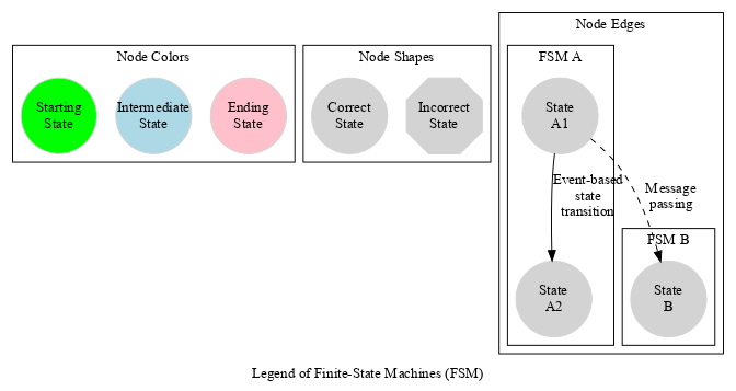
Not specifying an event condition on a state transition means here that the state change is time-based, i.e. it will occur automatically once a specific duration (in simulation time) will be elapsed.
The two models are interacting, thus the two FSMs will interact as well, based on message exchanges:

No inter-customer exchange is shown here: as an exercise, we could imagine that an impoverished customer may try to borrow money from another he knows.
So, from each of these FSMs, we can derive the behaviour of the corresponding model, from its initial logical state to all others. Transitions are clearly related to internal changes (e.g. the thirst of a customer builds over time - a.k.a. spontaneous behaviour) and external changes (denoted as the receiving of an actor message, like when a customer is notified of the price of a can of the vending machine.
Spontaneous Behaviour
The spontaneous behaviour describes how instances of a model behave, should their environment be fully passive. This behaviour is implemented in the actSpontaneous/1 [27] actor method, which takes the instance state as input and returns an updated one.
| [27] | As mentioned, the /1 means an arity of one, i.e. that this method takes only only parameter. More precisely, its type specification is -spec actSpontaneous( wooper:state() ) -> wooper:state().: the method is given a state, and shall return another one, possibly the same, possibly updated. |
For a customer like these ones, the spontaneous behaviour is rather simple: if he does not know yet the cost of a can, it requests it, otherwise it manages its thirst, i.e. it tries to order a can if the conditions are met.
The spontaneous behaviour of a soda vending machine is even simpler, as it is empty: modelled as they are, these machines are purely passive, nothing will happen unless their environment acts.
Other spontaneous behaviours might be considerably more complex: the normal, default mode of operation of, say, an incinerator could be very rich (with burners being driven, wastes being moved from a tank to another, etc.), not to mention the intents that could drive an human being.
Triggered Behaviour
Regardless of its spontaneous behaviour, a model instance can also develop a triggered behaviour, i.e. one that is specifically activated by other model instances, i.e. by the receiving of a corresponding actor message.
More precisely, any model (e.g. a cat one) can declare any number of signals (named actor oneways) that it may understand.
For example, a cat may be stroked, brushed, yelled at, fed, etc. Each signal (e.g. onBeingStroked) will lead to an actor oneway to be defined, to determine what the cat would do in this occasion. A cat being stroked can meow, purr, age twice as fast, explode, etc. depending on how we model it.
The definition of the function implementing an actor oneway includes at least two parameters: the first one specifies the state at which the instance receiving this message is, while the last parameter is a reference (a PID) onto the model instance which sent this signal. Between these two, any number of extra parameters can be listed (possibly none), so that that the signal can be fully described.
For a soda vending machine, a client inserting some coins corresponds to the sending of the orderSoda actor message, whose type specification is:
-spec orderSoda(wooper:state(),amount(),pid()) ->
                  class_Actor:actor_oneway_return().
We can see here that there is a single extra parameter, the exact amount of money the customer inserted. This will allow the machine to determine if:
- there is at least one can still in store (by reading the current can count in input state)
- the customer inserted enough money (by comparing the recorded can cost with the amount of money supplied, respectively in the actor input state and in the received actor message)
Based on that, the machine can determine whether a can must be sold. Then its returned state shall (corresponding to the oneway return) reflect the outcome, with one less can in store yet its amount of collected money being increased of the cost of a can.
Once having updated the state of its instance, this orderSoda/3 actor oneway shall also communicate back to the sender of the signal (here, a customer), so that it can know whether the transaction succeeded; here there are three possible outcomes:
- the transaction succeeded, the customer lost a bit of money (the cost of a can) yet gained a can - thus sooner being less thirsty
- the transaction failed and the customer remains as thristy as he was:
- either because there was no can left in the machine
- or because the customer did not insert enough money
How can the vending machine notify the customer of these outcomes? Simply by sending him back an actor message (among, respectively, getCan/2, onNoCanAvailable/2, or onNotEnoughMoney/2), using the PID listed as last parameter of the incoming actor oneway for that.
The union of all actor oneways declared by a model (the "signals" that can be triggered on it) constitutes the triggered behaviour of this model.
What's a Behaviour Anyway?
Typically any behaviour (be it spontaneous or triggered) boils down to any number of these actions:
- updating the instance state
- declaring that it should be spontaneously scheduled again in a specified future
- sending an actor message to other model instances (i.e. engaging an interaction)
- feeding a probe with result data
That's it!
Let's explain a bit further each of these terms.
Updating the state means having that actSpontaneous/1 or the triggered actor oneway (e.g. getCan/2) change the value of any attribute set in the state.
So a deterministic thirsty customer having succeeded in buying a can should have some way of keeping track of:
- the money he still has
- his level of thirst, i.e. in how much time he will be thirsty again
This may be done respectively with:
- a current_money attribute, of type amount(), a floating-point number of euros
- a next_thirsty_tick, of type class_TimeManager:tick_offset() that would be the next tick offset at which it will be thirsty again (more on these timing considerations later)
Or course other attributes will be useful to maintain a proper state of this deterministic customer:
- a reference onto the vending machine he knows (so that it can send actor messages to it): a known_machine_pid attribute, of type pid()
- the cost of a can (that the customer requested prior to any ordering attempt): an attribute named can_cost, of type amount() (for a given machine, the cost of a can being constant through the whole simulation, it is better to ask it once for all and to remember it, and then order repeatedly cans on that basis)
- the duration between the moment a can is drunk and the customer is thirsty again (repletion_duration, of type class_TimeManager:tick_offset()); for such a deterministic customer, it will be a constant
- whether a soda is being ordered (transaction_in_progress, of type boolean()) tells whether a transaction with a machine is in progress; it is necessary for the customer to remember that it started a buying attempt, otherwise, as the soda vending machine may take an arbitrarily long time to answer, it may order again and again a can before receiving its first feedback (i.e. actor message from the machine)
As mentioned, these deterministic customers are modelled so that they will be thirsty again once a fixed duration (in simulation time) elapsed since they drank their last soda can.
Implementing this behaviour is just a matter of:
- determining the repletion duration, in minutes, for the current deterministic customer; this is easy, as this is here a constant, specified amidst the construction parameters of these customers:
construct(State,[...],RepletionDuration,[...] ) ->
  [...]
- computing the number of ticks corresponding to this duration, by calling the class_Actor:convert_seconds_to_ticks/2 [28] function; in practice, as this fixed, high-level duration is known from the start, it can be converted once for all in a number of ticks directly from the constructor of the customer model (this cannot be statically, as the corresponding number of ticks depends on the simulation frequency separately set by the simulation case):
TickRepletionDuration = class_Actor:convert_seconds_to_ticks(
             60*RepletionDuration, ActorState ),
[...]
setAttributes( ActorState, [
    [...]
    {repletion_duration,TickRepletionDuration},
    [...]
                            ] ).
| [28] | The /2 designates an arity of 2, i.e. that this function takes two parameters, here the duration, in seconds, and the state of the instance. It would then return the duration expressed in simulation ticks. |
Then the repletion_duration attribute contains the number of ticks during which a deterministic customer will not be thirsty once he drank a can.
Currently, in the implementation of the thirsty customers, each instance is scheduled at each tick (as executeOneway(State,scheduleNextSpontaneousTick) is used), and the purpose of the repletion duration is only to establish whether, at some of these ticks, a soda can may be ordered.
Another implementation could have been to have thirsty customers be scheduled for a spontaneous behaviour only when they become thirsty again.
This could be done that way:
actSpontaneous(State) ->
  CurrentTick = class_Actor:get_current_tick(State),
  NextSpontaneousTick = CurrentTick + ?getAttr(repletion_duration),
  ScheduledState = executeOneway(State,addSpontaneousTick,
                                 NextSpontaneousTick),
  [...]
More real-life, complex examples can also be found in the City-Example case [29], for various models (Incinerator, IndustrialWasteSource, ResidentialWasteSource, Road, WasteTruck and WeatherCell). They all use the alternate, direct form class_Actor:add_spontaneous_tick/2 to perform their scheduling.
| [29] | Located in mock-simulators/city-example/src. |
These examples show how, in general (for spontaneous scheduling as well as for interactions) model-level durations can be expressed in their most general form (e.g. as mere seconds) yet can be easily converted in actual simulation ticks, in order to implement any kind of scheduling.
A special case is the request to schedule the next tick (scheduleNextSpontaneousTick/1), which may convey in some cases the notion of "immediate next step", rather than a duration as such.
However in this case the use of (diasca-based) interactions would generally be more appropriate, as they allow for arbitrarily complex exchange patterns to be performed - through multiple logical moments yet in the same tick (hence with no progress at all of the simulation clock).
Interaction
Unless mentioned otherwise, we consider that an interaction is to obey a specific timing.
For example, we can consider that communications (e.g. a customer speaking to another) are instantaneous, perceptions (e.g. a customer looking at a machine to read the cost of one of its cans, supposedly displayed on the machine) as well, but that other actions (e.g. a machine processing a can order) last for some model-specific duration (e.g. 800 ms of virtual time may elapse before a valid purchase results in a can being delivered to the corresponding customer).
The previous section showed how such timings should be expressed and used.
Note
As a rule of thumb: in a model, one should avoid expressing durations directly in terms of ticks; models shall be defined irrespective of any simulation frequency, as they may be involved in various simulations with various temporalities (as dictated by simulation cases).
One should thus use higher-level durations (e.g. expressed in seconds, or hours, etc.) and convert them in ticks only at runtime (possibly from constructors). All kinds of timings (for scheduling and interactions alike) can then be devised, knowing that, internally to models, ticks (as tick offsets) are the time units of choice for all processings.
State
Note
A discussion about constructors will be added here.
Defining Other Simulation Elements
Among the simulation elements that may be also defined in the context of a simulation, there are:
- command files
- scenarios
- special probes
- extra services
Let's discuss of these elements in turn.
Command Files
They allow to store the most common commands that are issued by the user in the context of this case. Typically, rather than typing the full command to executed said simulation, the user relies on a makefile (that we prefer to name GNUmakefile) that associated to a make target (e.g. batch) the actual command to be run (e.g. make city_benchmarking_run CMD_LINE_OPT="--batch").
As a result, the user may simply type from the command-line:
$ make batch
and have his simulation be run.
Scenarios
Scenarios, as discussed in the Sim-Diasca ontology [30], describe not the target city itself (this is the role of models) but its context (for example the weather system that may affect that city).
If, semantically, scenarios are very different from models, technically they are the same beasts: like a model, a scenario in the general case is constructed, has a state, may interact with others (be them scenarios or models), can produce results (thanks to probes), etc.
So, as an unexpected added bonus, you are already fully able to write your own scenarios!
| [30] | Please refer to the Sim-Diasca Technical Manual, section 3: "Let’s Start With A Short Ontology" for more information. |
Special Probes
Some projects may need to rely on specific data formats to express the simulation results.
For example, whereas Sim-Diasca generates natively time-series in a format that gnuplot can understand (see the class_Probe module) or that a Mnesia database can handle (see the class_DataLogger module), some projects may rely on a platform handling time series stored in a different format instead, like HDF5 or netcdf-4.
One solution is, if appropriate, to post-process the native Sim-Diasca result format in order to translate it to the format of choice. For the cases where it would not be feasible or straightforward, the best option is to write a custom probe, possibly relying on a binding to a library handling the target format.
An example of that is the class_CURTISProbe [31], which implements its own convention in terms of result storage and relies on a specific binding (allowing here to make use in this case of the well-known, standard HDF5 library).
| [31] | The CURTIS probe is a part of the sustainable-cities case, which is not provided with the free software version of Sim-Diasca (case for internal use only). |
Extra Services
Sim-Diasca provides generic services, yet more advanced simulations may require dedicated features.
For example, spatialised simulations have many geographic operations to perform, or simulation of a telecom system may have many domain-specific metrics like bandwidth and latency to compute.
These specific notions are not known of generic, lean and mean engines such as Sim-Diasca. Two main approaches allow to alleviate this issue:
- a bit like for the custom probes, already-existing, third party software elements can be reused to provide lacking services; for a spatialised simulation it would typically involve integrating a GIS (Geographic information system), possibly accessed to thanks to REST calls made from the models
- specialised layers can be defined between Sim-Diasca and the targeted models; for example, for the CLEVER project, a telecom layer was built on top of Sim-Diasca, providing base classes for all the related business-specific models (e.g. the layer was comprising notions of communicating device, network interfaces, packet router, etc.); then the domain-specific models could be defined more easily by re-using that adaptation layer, and could then directly manipulate bandwith, latency, routing elements, etc.
Conclusion
By going through this modelling guide, we recreated elements of an example of a simulation that actually exists, and can be found in the free software version of Sim-Diasca. The full code of this example case is indeed located in mock-simulators/soda-test/src.
More advanced users are advised to have a look also to the City-Example case, located in mock-simulators/city-example/src, for a considerably more complex and demanding example case.
We hope that writing simulations will be easier thanks to the examples provided with the Sim-Diasca code base and thanks to this guide oriented towards modellers.
As always, any (constructive!) feedback is welcome (for that use the email address at the top of this document). Should some point remain unclear, please feel free to contact us, as we try to provide support on a best-effort basis.