Sim-Diasca Dataflow HOWTO

![]()
![]()
| Organisation: | Copyright (C) 2016-2025 EDF R&D |
|---|---|
| Contact: | olivier (dot) boudeville (at) edf (dot) fr |
| Authors: | Olivier Boudeville, Samuel Thiriot |
| Creation Date: | Thursday, February 25, 2016 |
| Lastly updated: | Friday, July 18, 2025 |
| Version: | 2.4.8 |
| Status: | Stable |
| Website: | http://sim-diasca.com |
| Dedication: | For the implementers for Sim-Diasca dataflow-based models. |
| Abstract: | This document describes how dataflows, i.e. data-driven graphs of blocks, are to be defined and evaluated in the Sim-Diasca simulations relying on them. |
Table of Contents
- Foreword
- Usual Organization of the Model Evaluation
- An Alternate Mode of Operation: the Dataflow
- On Dataflows & Experiments
- On Dataflow Processing Units
- On Dataflow Ports, Channels and Buses
- On Dataflow Values
- Logic of the Dataflow Block Activation
- On Dataflow Objects
- On Model Assemblies
- A More Complete Example
- Developing Dataflow Elements in Other Programming Languages
- More Advanced Dataflow Uses
- Experiments
- A General View on the Dataflow Synchronisation
- The World Manager and its Dataflow Object Managers
- The Experiment Manager and its Unit Managers
- About Mock-up Units
- Integrating a Model As a Dataflow: a Short Walkthrough
- Preliminary Step (#0): Remembering the Basics
- Step #1: Ensure that the Overall Simulated World Can be Structured As a Dataflow
- Step #2: Determine the Specific Relationships Between the Dataflow and this Model
- Step #3: Break the Black Box Into Actual Dataflow Units
- Step #4: Implement the Corresponding Actual Units
- Step #5: Add the Corresponding Unit Manager(s)
- Requirements For the Dataflow Integration of a Model
- Implementation Section
- Appendices
Foreword
The simulation of complex systems often relies on loosely-coupled agents exchanging signals based on a dynamic, potentially complex applicative protocol over a very flexible scheduling.
However, in some cases, the modelling activity results alternatively in the computations being at least partly described as a static network of interconnected tasks that can send values to each other over channels that applies to a simulated world - i.e. a dataflow.
Both approaches will be detailed and contrasted below, before focusing on how dataflows can be defined and used with Sim-Diasca.
Note
Most of the dataflow-related concepts mentioned in this document are illustrated on a complete, runnable simulation case: the Dataflow Urban Example, whose sources are located in the mock-simulators/dataflow-urban-example directory of the standard Sim-Diasca distribution.
Besides these case-specific elements, the sources of the generic dataflow infrastructure are also available, in the sim-diasca/src/core/src/dataflow directory.
Please feel free to skim in these respective sources for a better practical understanding of the dataflow infrastructure.
Usual Organization of the Model Evaluation
In most simulations of complex systems, the simulated world is sufficiently disaggregated into numerous autonomous model instances (be they named agents or actors) so that the evaluation of their respective behaviours and interactions naturally leads to processing the simulation. In this context, trying to constrain or even hard-code static sequences of events is often neither possible nor desirable.
For example, one can see a city as a set of buildings, roads, people, etc., each with its own state and behaviour, the overall city (including its districts, precincts, etc.) being the byproduct of their varied interactions - a possibly hierarchical, certainly emergent organisation.
This approach is probably the most commonly used when modelling a complex system, hence it is the one natively supported by Sim-Diasca: the target system is meant to be described as a (potentially large) collection of model instances (a.k.a. actors) possibly affected by scenarios and, provided that their respective state and behaviour have been adequately modelled, the engine is able to evaluate them in the course of the simulation, concurrently, while actors feed the probes that are needed in order to generate the intended results.
The (engine-synchronised) interactions between actors are at the very core of these simulations, which are determined by how actors get to know each other, exchange information, opt for a course of action, create or destroy others and, more generally, interact through an implicit overall applicative protocol resulting from the superposition of their individual, respective behaviours.
However other, quite different, organisational schemes can be devised, including the one discussed in this section, the dataflow paradigm.
An Alternate Mode of Operation: the Dataflow
Let's define first what is a dataflow.
Note
A dataflow is a way of describing a set of interdependent processings whose evaluation is driven by the availability of the data they are to handle.
In this more constrained organisation, rather than having actors freely exchanging various symbols and messages according to dynamically-decided patterns, we rely here on quite specialised actors that embody dataflow blocks, which are:
- either dataflow processing units (instances of the DataflowProcessingUnit class), which set and listen for values, through channels that are delimited each by an input port and an output port, and perform associated computations
- or dataflow objects (instances of the DataflowObject class) that stores attributes that can be set and read respectively thanks to their associated input and output ports
All these dataflow blocks and the channels linking them form altogether a graph (whose nodes are the blocks, and whose edges are the channels). This graph is by default:
- statically defined: its structure can be established before the simulation starts
- static: in the general case, its structure is not expected to change in the course of the simulation
- directed: channels are unidirectional, only from an output port of a block to an input port of a block
- acyclic: by following the declared (directed) channels, no path should go through the same block more than once
The graph can be explicit or not: either it is described as a whole (as a single, standalone entity), or it can be merely extrapolated from the union of the channels drawn between the declared blocks.
Dataflows of course have an immediate graphical counterpart. The conventional symbols we elected are represented in this key:
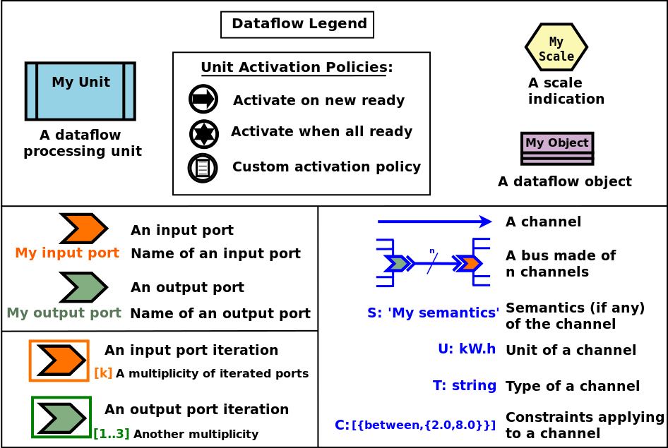
By convention, input ports are in orange, output ports in green, dataflow objects in light purple, dataflow units (e.g. processing or mock-up ones) are in light blue and comprise the symbol of their activation policy, and channels are in various shades of blue [1].
| [1] | Please refer to Annex 3: Conventions for the Graphical Representation of Dataflows for more information. |
Still in blue, the SUTC quadruplet:
- the channel Semantics (i.e. the meaning of the conveyed values) can be specified, as an arbitrary domain-specific symbol prefixed with "S:" (like in "S: 'produced heat'"); project conventions may apply, notably in order to adopt the RDF format, like in:
S:'http://foobar.org/urban/1.1/energy/demand'
- the Unit of the value, prefixed with "U:" (e.g. "U: kW.h", or "U: g/Gmol.s^-2"); often the unit information implies a type (described in next point): for example the unit "U: W" implies the type "T: float"; in this case the type information can be safely omitted
- the Type of the values conveyed by the channel, prefixed with "T:" (e.g. "T: string" or "T: {integer,boolean}")
- the Constraints (if any) applying to the exchanged value, as a list of elementary constraints (e.g. "C: [ {between,{2.0,8.0}} ]" means that a single constraint applies to the exchanged values, which is that they must be between 2 and 8)
These SUTC information shall preferably be specified close to the associated channel (if any) or output port.
Unit activation, semantics, units, types and constraints are discussed more in-depth later in this document.
Specifying the names of dataflow units and ports is mandatory.
As a processing unit is in charge of performing a specific task included in a more general computation graph (the dataflow), its name shall reflect that; one may consider that the name of such a unit is implicitly prefixed with a verb like compute_. For example, a processing unit named fuel_intake could be understood as compute_fuel_intake (and we expect it to have at least one output port dealing with fuel intake).
Finally, as some dataflow units have for purpose to aggregate metrics across time and/or space, some scale indication may be given for documentation purposes, enclosed in an hexagon in pale yellow.
The dataflow objects are specifically discussed in a section of their own later in this document.
As a result, a dataflow, which shall be interpreted as a graph of computations, may look as this (meaningless) example:
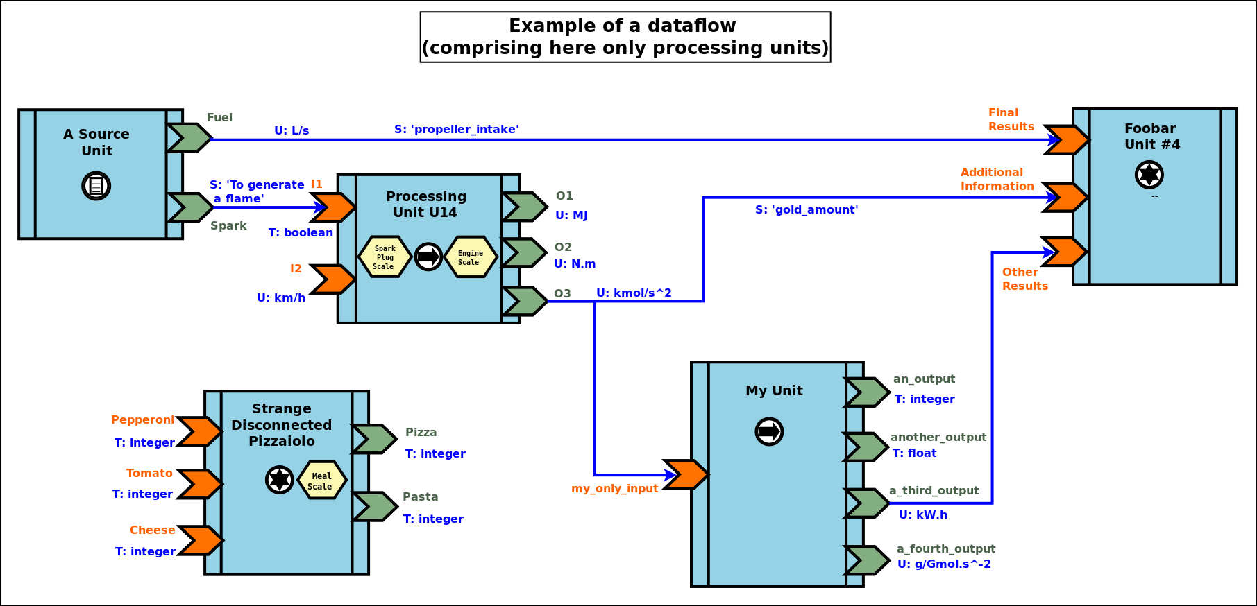
We can see that a dataflow does not need to be fully connected (the blocks may form disjoint subgraphs) and that ports (input and output ones alike) may not be connected either.
The global progress of the computations happens here from left to right.
A more complete example is given later in this document.
Now let's detail a bit all the elements involved.
On Dataflows & Experiments
Dataflow Definition
As mentioned, a dataflow is a graph of computations whose evaluation is driven by the availability of the data they are to handle.
In practice, it is a set of interlinked dataflow blocks, typically dataflow processing units and dataflow objects.
Even though dataflows could remain only implicit data-structures (they would just correspond to an actual set of interlinked dataflow elements), we preferred introducing an actual dataflow class, in order to ease the interaction with such instances and provide a reference point.
So overall operations on a given dataflow (e.g. creations, modifications, report inquiries) shall be operated only through its corresponding federating class_Dataflow instance.
Multiple dataflow instances may exist, and they are collectively managed by the overall experiment manager, introduced later in this document.
Experiment Definition
An experiment corresponds to the overall evaluation task that is to be performed by a (here: dataflow-based) simulation, as it is described by the corresponding simulation case.
For that such an experiment aggregates any number of dataflows, which progress in parallel, typically through a series of steps [2].
During each step, each dataflow instance, based on any update of its input ports, is fully evaluated (i.e. until it reaches a fully stable state).
| [2] | In engine-related terms, an experiment step of the dataflow infrastructure corresponds to a simulation tick of the engine. During such a step, dataflows are evaluated over diascas, resulting on their elements exchanging values, until none of the output port is set anymore. Then the next step (tick) can be evaluated, etc. |
More in-depth information can be found in the Experiments section.
On Dataflow Processing Units
A (processing) unit is, with dataflow objects, the most common type of dataflow block.
A dataflow unit encapsulates a kind of computation. For example, if an energy demand has to be computed in a dataflow, an EnergyDemandUnit processing unit can be defined.
Such a unit is a type, in the sense that it is an abstract blueprint that shall be instantiated in order to rely on actual units to perform the expected computations. Therefore, in our example, a class_EnergyDemandUnit processing unit shall be defined (specified and implemented), so that we can obtain various unit instances out of it in order to populate our dataflow.
As discussed in the next section, each of the instances of a given dataflow unit defines input and output ports.
Note
It shall be noted that, additionally, each processing unit instance benefits from a state of its own (that it may or may not use): the attributes that the unit class introduced are available in order to implement any memory needed by the unit, and of course these attributes will retain their values through the whole lifetime of that instance (hence through simulation ticks and diascas).
So a unit may encapsulate any processing between a pure, stateless function to a more autonomous, stateful, agent.
On Dataflow Ports, Channels and Buses
A port is the only way by which a dataflow block (typically a unit) may interact (propagate a value) with other blocks.
Following rules apply:
- a port is either an input one (listening to the update of a value conveyed by the corresponding channel) or an output one (able to update its corresponding value and notify its registered input listeners); this is reflected by their type (either input_port or output_port)
- each port is named (as a non-empty string [3], e.g. "my foobar port") and no two input ports of a block can bear the same name, nor output ones can (however an input port and an output port of the same block can have the same name - they will be differentiated by their nature)
- a port identifier is defined from a pair made of an identifier of the block that defined it and from the name of that port [4] (e.g. it could be ("My Unit","Port 24"), or based on more technical identifiers)
- a port (input or output) may either hold a value (arbitrary data can be set; the port is then considered as ready, i.e. as set), or not - in which case it holds the unset symbol (the port is then itself considered as unset)
- an output port can be considered as being always unset: as soon as a new value is available, it notifies all its connected input ports and then reverts back to the unset status; therefore the set/unset status can be abstracted out for output ports, which just get punctually activated
- conversely, this status matters for input ports: a block starts with all its input ports to unset, and, each time an input port is notified by an output port, this input port switches to set; how a block is to react depending on none, one, some or all of its input ports being set is discussed below
- an output port will send downstream the value it holds whenever:
- it gets set: exactly one sending will be performed per setting (regardless of the value that is set) to each of the input ports it is linked to; as a result, setting explicitly a port to a value that happens to be the same as the one that it was already holding will nevertheless trigger a sending (therefore "not setting a value" vs "setting the current value again" are operations that differ semantically)
- it gets connected (i.e. a channel is created from this output port to an input port) whereas this output port has already been set at least once in the past; then, on channel creation, the latest value it sent will be re-emitted, only to the newly connected input port
- ports can convey arbitrary data (i.e. any Erlang term), yet any given port has a type, which defines what are the licit the values that it can hold (e.g. "this port can be set to any pair of non-negative floats") [5]
- a block can declare any number of output ports (possibly none, in which case it is an exit block, a sink)
- a block can declare any number of input ports (possibly none, in which case it is an entry block, a source)
- a channel links exactly one output port to one input port, and these two ports shall have the same types, units and semantics (which are the ones of the channel)
- any number of channels may originate from an output port (possibly none); when an output port is being set (i.e. when it performs a punctual transition from unset to set), then all the input ports listening to it are notified of that [6]
- an input port may be the target of up to one channel; if no channel feeds a port, then it remains in the unset state
- a port records the timestamp (in simulation time) of the last notification (possibly none) it either sent (for output ports) or received (for input ones)
- a bus corresponds to a set of channels ; it shall be seen, at least currently, only as a graphical convention introduced in order to avoid that too many parallel channels are drawn, which would obfuscate the representation of a dataflow (note that no bus per se is considered when evaluating the dataflow; the runtime is only aware of ports being connected to others, so buses - and even channels - are abstracted out)
| [3] | The only restriction is that the "_iterated_" substring cannot exist in a user-defined port name (so for example "foo_iterated_bar_42" will be rejected by the dataflow infrastructure). |
| [4] | A port identifier is typed as -type port_id() :: {dataflow_object_pid(),port_name()}. where dataflow_object_pid() is a PID (the one of the block) and port_name() is a binary string. |
| [5] | The dataflow system may or may not check that typing information. |
| [6] | Indeed the onInputPortSet/3 actor oneway of their respective block is executed, specifying the port identifier of the triggered input port and the corresponding timestamped value (specifying the tick and diasca of the notification). Generally this information is not of interest for the block implementer, as defining for example a unit activation policy allows to handle automatically input ports being triggered. |
Even if conceptually it is sufficient that only the output port knows the input ports it may notify (and not the other way round), technically the input ports also know the (single, if any) output port that may notify them, for example for a simpler support of unsubscribing schemes.
On Dataflow Values
We saw that a value designates a piece of data carried by a channel, from an output port to any number of input ports.
Various information are associated to the output ports and to the values they carry (they are metadata), notably the SUTC quadruplet (for Semantics-Units-Type-Constraints), which the next sections detail in turn, yet in a different order for the sake of clarity - roughly from the most concrete to the highest-level.
Type of a Value
Type Basics
A channel is typed, in the sense that all the values that it conveys shall be of the same type (in terms of programming language; e.g. a floating-point value), which is the one specified for the channel. The T in SUTC stands for this type information.
The name of a type must be a series of alphanumerical characters, in lowercase, starting with an alphabetical one, and possibly containing underscore (_) characters; example of a type name: integer or this_is_my_type_name_221.
The complete type specification in a dataflow (typically used to describe a port) shall be prefixed with "T:" (for example "T: integer" would mean that the corresponding port handles values of type integer).
In the absence of unit information (see next section), the type information is mandatory and must be specified by both port endpoints. It may or may not be checked, at build and/or run time.
Note
The specified typing information is currently not used: as a consequence, the values conveyed by the dataflow are not yet checked against their declared type.
A set of built-in and derived types is provided, and many port specifications rely directly on them in order to define simple, scalar, atomic values (often floating-point ones) - as opposed to compound ones. Specifications may also define and use any additional type that they may need.
Moreover, if deemed useful, more complex data structures may be specified, based on polymorphic types like tuples (denoted as {}), on lists (denoted as []) or even, in the future, on associative tables.
All these constructs enable the specification of all the typing information needed by the user in order to describe, in computing terms, the values exchanged over the dataflow.
Let's discuss the basic typing primitives first, i.e. the built-in types.
Built-in Types
Following built-in types are available (they map to Erlang native types; some related technical details put between parentheses or in footnotes may be safely ignored by the reader):
| Name of the built-in type | Description | Example value |
|---|---|---|
| integer | Any (unbounded; positive or negative) integer value. | -112 |
| float | Any floating-point value (in double precision). | 3.14159 |
| number | Any number (either an integer or a float) [7]. | 1.1 |
| string | Any series of characters delimited by double quotes [8]. | "Hello world!" |
| boolean | Either 'true' or 'false'. | 'true' |
| count | A non-negative integer, to mention a number of elements (possibly zero). | 17 |
| percent | A floating-point percentage (alias of float), the value 1.0 corresponding to 100%. | -1.4 |
| json_content | An opaque, stringified JSON representation of a value. | (undisclosed, as meant to be opaque) |
| any | Wildcard type, corresponding to any type (no information given, hence no type checking can be performed in this case). | "I am a value." |
| [7] | Note that some types overlap, notably some of them are special cases of others, like integers and numbers. So, for a given value, multiple type specifications apply (e.g. any will always match). |
| [8] | Mapped as an Erlang binary string, displayed as a basic string. |
Note
Indiscriminate use of the any type is strictly prohibited; typically it should never be used operationally (e.g. when defining actual ports), as it would then be a way of bypassing the type system.
For advanced users: the main use of any lies in the very specific context of "polymorphic units", i.e. units that may be able to process values of all kinds of types.
Derived Types
These types are not built-in, they are to be specifically derived (possibly by the user directly) from other types (which themselves may be built-in or derived).
Type Definition
Often, a new type definition has to be used in several occurrences (e.g. when having different ports that happen to rely on the same type). Rather than repeating the same type definition each time, we recommend that, as soon as a type definition is used more than once for the same purpose, a (derived) type is defined from it and named one time for all - and then referred to as often as needed.
Indeed, being (new) types, derived types have their own name (e.g. my_own_type), knowing that the names of all built-in types are reserved.
So, in order to define a derived type named my_own_type according to any kind of definition (designated here by A_TYPE_DEFINITION), the following syntax shall be used:
my_own_type :: A_TYPE_DEFINITION
For example, if various ports had to handle a number of vehicles, then it may be advisable to introduce a specific type for this purpose, which could be named vehicle_count.
In this case, this derived type would happen to be simply a synonym of the integer built-in type (the vehicle_count type would then be here an alias a the integer built-in one):
vehicle_count :: integer
Then, this new type being defined, ports may use it and specify that they handle channel values of that type, thanks to T: vehicle_count.
Type Constructs
Aliases are of course useful, yet one may have to specify types that are more complex than exact synonyms of the built-in types.
For that, the user can rely on following type constructs, which allow introducing new types, or combinations thereof:
union types, i.e. types that regroup other types and whose values can be of either one of these types
- in the specification of such an union type, the listed types are separated by the pipe (|) character, representing the OR operator
- for example, the union of types T1, T2 and T3 is: T1|T2|T3; the aforementioned number built-in type can be defined as: integer|float
symbol types, each of which being a simple label (a non-empty series of characters delimited by single quotes), like 'my_symbol' or 'Red Alert'; a symbol is both a type and a value, in the sense that defining a symbol is defining a type which happens to have a single value (itself) [9]; moreover type names are themselves symbols (without their single quotes); so defining my_type as, for example, integer, corresponds to the definition of an alias type, a synonym of integer which can be used in other type definitions (such as in [my_type])
enumerated types (a.k.a. enumerations) is a user-defined union of symbols, simply obtained from the two previous constructs; for example a burner_status enumeration type might be defined as:
'burner_enabled' | 'burner_disabled' | 'burner_on_operation'
and a value of that type (a symbol) may be, for example: 'burner_disabled'
One can see that the boolean type is actually nothing but a 'true'|'false' enumeration.
Defining a single-type enumeration corresponds to defining a symbol type.
| [9] | Symbols are mapped to Erlang atoms. |
Polymorphic Types
Finally, in addition to all the atomic types (built-in or derived) presented above, following built-in polymorphic types (types that depend on others) are supported as well:
- list of type T, noted as list(T) or [T]: any kind of (proper, homogeneous) list (empty or not), represented between square brackets, to account for a variable-size sequential container containing values of type T
- e.g. list(integer) and [integer] denote the same type, a list containing any number of integers; values of that type can thus be: [4,-17], [], etc.
- list() refers to any kind of list (alias of list(any))
- tuple containing elements of types T1, T2, T3, etc., noted as {T1,T2,T3,...}: any kind of tuple (fixed-size container, homogeneous or not), delimited by curly braces
- e.g. a value of the {burner_status,float,[bool]} type might be {'burner_on_operation',14.7,['false','false']}
- tuple(T) refers to tuples whose elements are all of type T, and whose number is not specified (e.g. {2,46,5} is of type tuple(integer)), while tuple() refers to any kind of tuple
- in later versions: associative tables, whose keys are of type Tk and values are of type Tv, noted as table(Tk,Tv)
Note that recursive types (e.g. a type tree being defined as {tree,tree,node_content}), are, at least currently, not allowed (they can be expressed yet no specific support for them is provided).
Implementation-wise
The dataflow infrastructure includes a TypeServer, which tracks statically (i.e. on a per-class level) or dynamically (for any dynamically-created port) the type declarations and uses, to provide a first, very basic support for typing enforcement.
Unit of a Value
A value of a given type (typically a float) can actually correspond to quantities as different as meters and kilowatts per hour.
Therefore units shall preferably be specified alongside with values, and a language to express these units must be retained. The U in SUTC stands for this unit information.
One should refer to the documentation of the Myriad layer [10] for a description of how units can be specified, compared, checked and used.
| [10] | Please refer to the Description of the Management of Units section, in the technical manual of the Myriad layer (in Ceylan-Myriad-Layer-technical-manual-english.pdf). |
In a dataflow, the unit of the values that will be held by a port shall preferably be specified when declaring that port. This is done thanks to a string, prefixed with "U:" (e.g. "U: kW.h", "U: g/Gmol.s^-2" or "U: {mm,mm,mm}" for a 3D vector in millimeters).
Specifying the unit of a scalar value implies declaring its type as float.
If, for a value, no unit is given, then its type, as discussed in Type of a Value, shall be specified.
Semantics of a Value
Specifying the type and unit of a value is certainly useful, yet it would generally be insufficient to convey its meaning, i.e. to express how that value shall be interpreted.
For example, knowing that a port accepts floating-point values in kilojoules does not tell whether this value corresponds to an energy demand, an actual consumption or a production.
Therefore this domain-specific information shall be specified separately. It is to be done thanks to the specification of a symbol (similar to a string, corresponding to an Erlang atom), prefixed with "S:", standing for semantics (which is the S in SUTC). For example: "S: 'security credentials'" or "S: 'energy_demand'".
We recommend that semantics are specified according to a well-defined, standard format: RDF (standing for Resource Description Framework).
RDF statements (potentially expressed as RDF triples) about subjects (e.g. a block or a port) clarify the intents (made them explicit and expressed in an uniform way) and may allow the use of tools able to perform queries and inference. This may enable, in the future, the automatic checking and even generation of proper dataflows.
Typically a port semantics is then a subject in RDF parlance, like in:
S:'http://foobar.org/urban/1.1/energy/demand'
where:
- the normalising organisation is designated by its domain name foobar.org
- it published a urban ontology, whose version in use here is 1.1
- it addresses potentially multiple fields of interest, including the one of energy
- one sub-topic of which is the demand (of energy)
As a result, the full chain (the output port, the channels, the value itself and the related input ports) can perform a basic check of the semantic consistency for each exchange over the dataflow, and have an extra chance of detecting and rejecting any erroneous port connection (even if in technical terms, i.e. in terms of typing and unit, it may look perfectly legit).
Currently a minimum lexicographic distance (the Levenshtein one) is enforced (by the SemanticServer of the dataflow infrastructure) between any two semantic elements, so that any spelling mistake can be more easily detected.
Generally the channel is shown as bearing the semantics, implying that this formalised meaning is shared by the corresponding output port, the associated input ports and by the values that they exchange.
Constraints Applying to a Value
The C in SUTC stands for this constraints information.
They allow to specify a set of rules by which the value must abide.
Note
Unlike most of the other meta-data (e.g. semantics or type), constraints are not considered as being intrinsic to a value; they are generally seen as a property (on values) that is enforced at the port level.
The following constraints can be mixed and matched:
- {greater_than,G} means that the (scalar) value must be greater than, or equal to, the number G
- {lower_than,L} means that the (scalar) value must be lower than, or equal to, the number L
- {between,A,B} means that the (scalar) value must be greater than, or equal to, the number A and lower than, or equal to, the number B
- {in,L} means that the value must be an element of the list L
- positive means that the (scalar) value must be positive (possibly null)
- strictly_positive means that the (scalar) value must be strictly positive (null not allowed)
- negative means that the (scalar) value must be negative (possibly null)
- strictly_negative means that the (scalar) value must be strictly negative (null not allowed)
- non_null means that the (scalar) value must not be null (strictly positive or negative, zero not allowed)
For example, constraints applying to a value could be:
C: [ {between,2020,2040}, {in, [1989,2021,2030,2988]} ]
Note
As mentioned, for all numerical comparisons (e.g. greater_than), the value of interest is expected to be a (scalar) number.
Otherwise (e.g. the value is a triplet, or the value is not a number), the associated constraint is considered as not satisfied.
All constraints have to apply (as if they were associated by AND operators). The previous example would thus allow only two possible values, 2021 and 2030.
Various additional kinds of constraints may be supported, based on encountered needs.
Constraints are currently parametrised by constants (e.g. {greather_than,10.0}); maybe in the future they could also accept references onto other local ports (e.g. to compare their values or base some constraints on operations, like sum, performed on their values).
Accuracy of a Value
This may be the next value-level metadata to be handled by the dataflow infrastructure.
Depending on various factors like data quality and numerical errors (e.g. floating-point rounding), the computed values might show a good precision and many digits, yet a poor accuracy.
The first step to prevent it is to measure how accurate a computation is. This can be evaluated thanks to relative error and ulps (for units in the last place).
So an accuracy may be associated to each value exchanged over the dataflow, and it may then be updated by each processing unit relying on it.
By default accuracy is best measured in terms of relative error, as, if ulps are the most natural way to measure rounding error, they are less suitable to analyse the error caused by various formulas.
Anyway, often only the order of magnitude of rounding errors is of interest, and ulps and relative errors may be used interchangeably since their magnitude differ by at most a constant factor, the radix, typically equal to 2 (binary representation), or less frequently 10 (decimal one).
Another measure could be the "precision", once defined as the number of bits used to represent the significand of a floating-point number. Libraries like MPFR can be given a target, arbitrary precision and may enforce it (hence we would expect the accuracy of the corresponding values to be constant across the corresponding ports).
Each project is free to retain its own conventions regarding how the accuracy is quantified (usually as a floating-point number). The dataflow infrastructure provides the mechanisms to keep track of it, and, in processing units, update it. An accuracy specification is to be prefixed with "A:", like in "A: 8".
Should no accuracy be used for a given value, it should be replaced by the 'unknown_accuracy' atom (which is the default).
The accuracy could be also translated as a confidence interval, i.e. an interval that covers an unknown parameter with probability P=1-alpha, where P is the confidence level, and alpha should be as close as possibly to 0 (typical values of P: 0.95, 0.99 or 0.999) thanks to a sufficiently large number of samples.
As no general consensus exists about accuracy, it has not been included among the usual metadata associated to values. In the future this could added, accuracy becoming the A of SUTCA.
Wrapping Up About Values
So an output port may send a notification to a set of input ports, with the following information being associated:
- a semantics, like in S: 'energy_demand'
- a unit, like in U: kW.h
- a type, like in T: float
- constraints, like in C: [{lower_than,100}]
- an accuracy, like in A: 11.0, to be understood here as the number of bits for the precision of the significand
- a value, like in 6.7121
- a timestamp, like in {117,3}, i.e. tick offset #117, diasca 3
- the port identifier of the sender
The semantics, the unit, the type carried by endpoints and the sender port identifier are exchanged and checked at the channel creation, i.e. when the input port is linked to its output one.
The unit of the value, its associated constraints, its accuracy, its actual value and its timestamp are checked and sent to the input port each time it is triggered by its output port.
Logic of the Dataflow Block Activation
We saw that a key element of a dataflow lies in its blocks, notably in its processing units.
Note
Blocks are either dataflow objects or dataflow units. We will discuss here mainly of the latter (i.e., of units), as the activation of a dataflow object offers no flexibility: it will be activated iff at least one of its input ports has been assigned, leading to its corresponding attribute(s) being set, and to the associated outport(s) being in turn assigned.
For a given dataflow block, it must be decided:
- at which logical step the block is to be activated, i.e. when the activation of a block shall be examined
- on which additional condition(s) it shall be activated, i.e. how in practice the block update shall be determined as having to be triggered
- what results from such an activation, i.e. what are the operations this block should then perform
Such an activation translates to the execution of the activate/1 method of that block (at this point, it is most probably a processing unit). The role of this method is to be the place where the unit defines its actual processing; for that, the unit most probably overrode the corresponding default do-nothing implementation.
During this processing, as for any actor oneway, the unit is free to perform computations, to send actor messages and to operate state changes. This includes notably reverting any of its input ports to the unset state, and activating any of its output ports.
Now that it has been determined what an activation entails (pretty much anything within the degrees of freedom of an actor), the conditions ruling when an activation shall occur are to be specified. Various policies are available for that.
For a given activation policy, these conditions should only depend on the readiness of the input ports of that unit, and of its state.
Even if a given processing unit might define its own activation rules, the set of built-in activation policies described below should be sufficient for most uses.
In all cases, under the hood the unit will be notified thanks to an actor message that one of its input ports has been triggered, knowing that during a diasca any number of such messages may be received (indeed a unit may have multiple input ports; moreover, even if it may not be usual practice, an upstream block might have triggered one of its output ports more than once) and then reordered before being processed on the next diasca.
The 'Activate On New Set' Policy
The first built-in activation policy consists in updating the unit when at least one of its input ports went from unset to set.
This policy, named activate_on_new_set, will activate the unit at most once per diasca, at the one immediately following the diasca at which these input ports were triggered, no matter of how many input ports were triggered on the previous diasca nor on how many times they were each triggered.
An (unordered) list of input port triggers, together with the corresponding values then set, will be available to the activate/1 method when it will be automatically executed.
Either a bulk update may follow (the unit taking them into account as a whole), or it may perform a fold on that list to react in turn to each trigger (to emulate the case where they would be received and processed one after the other [11]).
| [11] | Note that, as all actor messages, the triggers have been reordered by the engine according to the simulation mode. |
It is up to the unit to reset the input ports (i.e. to set each of them back to the unset state) when deemed appropriate.

This Activate On New Set policy (sometimes shortened as the "On New" policy) is graphically symbolized as an arrow, to denote that any update of an input port directly triggers the associated unit computation.
The 'Activate When All Set' Policy
The second built-in activation policy, named activate_when_all_set, is to update the unit if and only if all of its input ports have been set: each time an input port is triggered, this policy automatically determines if it was the last one still unset and, if yes, it executes the activate/1 method.
Note
This policy used also to take care, once that method had been executed, of automatically setting back all input ports to their unset state.
As at least some models rely on "stable" inputs (inputs that vary infrequently, if ever - and thus may be set only once, but read multiple times), we preferred disabling that mechanism. So, now, in all cases, input ports are never automatically unset.

This Activate When All Set policy (sometimes shortened as the "When All" policy) is graphically symbolized as a star resembling to a lock, to denote that no associated unit computation will take place until all input ports have been enabled (i.e. are set).
Custom Activation Policies
Some units may require, under rare circumstances, a custom policy, i.e. a policy of their own that does not match any of the built-in ones.
For example source units, i.e. units not having any input port, can be defined, but of course then none of the policies above can apply (as they can never be triggered). Nevertheless such source units are typically needed in order to bootstrap the processing of a dataflow.
To solve this, rather than forcing the definition of at least one "dummy" input port per unit, all units can also be explicitly triggered: they can rely on their activateExplicitly/2 actor oneway for that, in charge of calling their activate/1 oneway as other policies do.
This policy may for example also be used to account for units having fixed, active temporalities. A daily-activated unit may schedule itself every 24 hours (declaring such a regular spontaneous scheduling, during which it may activate its output ports), while another unit may be ruled per-hour.
So dataflows can federate mixed temporalities, knowing that the use of this policy of explicit activation is fully optional (as by default a dataflow is fully passive and is only driven by changes in its input ports) and shall be regarded only as a last resort, should the built-in policies be insufficient.

This Custom policy is graphically symbolized as a sheet of paper, to denote that the unit activation is driven by a freely chosen user-specified logic.
On Dataflow Objects
We asserted previously that the most common form of dataflow block is the processing unit; the other major form is the dataflow object, discussed here.
Indeed, if dataflow units allow to describe the computations that shall be performed, generally they have to rely on the structure of the simulated world in order to feed their computations with relevant data.
Holding these information, and possibly making them change over time, is the purpose of the dataflow objects. They are plain, standard (Sim-Diasca) actors, except that they may define dataflow attributes, i.e. their own state attributes that can be involved in dataflows.
To a dataflow attribute is indeed generally associated a pair of ports, an input one and an output one. These ports allow to bridge the gap between two worlds:
- the one of the multi-agent, dynamic, loosely coupled actors, serving the purpose of describing a disaggregated target system and its evolution
- the one of the (mostly statically connected) dataflow units, in charge of performing computations over a target system
A dataflow object is represented with the light-blue background that is common to all dataflow blocks, while each of its attributes is associated to an input and/or an output port (typically both), like in:
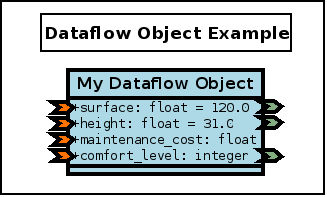
In this example, all attributes are standard, "bidirectional" attributes (they can be read and/or written by other dataflow blocks), except the maintenance cost, which is a "terminal" attribute (in the sense that it can be set, yet cannot be read by other blocks of the dataflow).
On Model Assemblies
Defining the Notion of Assembly
As seen already, within simulations, the target system (e.g. a city) is translated into a set of instances of dataflow objects of various types (e.g. Building, Household, etc.), on which models - themselves made of a set of instances of processing units of various types (e.g. EnergyDemand, PollutionExhausted, etc.), complemented with at least one unit manager - are to operate.
The (generally interconnected) set of models involved into a single simulation is named a model assembly.
Assemblies may comprise any number of models: generally at least one, most often multiple ones, since the purpose of this dataflow approach is to perform model coupling.
Let's from now adopt the convention that a model name is a series of alphanumerical characters (e.g. FoobarBazv2) and that its canonical name is the lowercase version of it (e.g. foobarbazv2).
Ad-hoc Assemblies
One option is that a FoobarBazv2 model is directly integrated in a dataflow thanks to an ad-hoc simulation case for a target assembly, a case whose name could be freely chosen (e.g. my_foobarbazv2_case.erl).
Then, in this simulation case (accounting for the corresponding assembly), all relevant FoobarBazv2-specific settings would have to be directly specified (e.g. the elements to deploy for it, the unit managers it is to rely on, etc.); note that these model-specific information would be somewhat hardcoded there.
Dynamic, Composable Assemblies
Alternatively, rather than potentially duplicating these settings in all cases including that model, one may define instead a foobarbazv2-model.info file (note the use of its canonical name) that would centralise all the settings relevant for that model, in the Erlang term format [12].
For example it could result in this file having for content (note that these settings can be specified in any order):
% The elements specific to FoobarBazv2 that shall be deployed:
{ elements_to_deploy, [ { "../csv/Foobar/Baz/version-2", data },
                        { "../models/Foobar-Baz", code } ] }.

% To locate any Python module accounting for a processing unit:
{ language_bindings, [ { python, [ "my-project/Foobar-Baz/v2" ] } ] }.

% Here this model relies on two unit managers:
{ unit_managers, [ class_FoobarBazEnergyUnitManager,
                   class_FoobarBazPollutionUnitManager ] }.
| [12] | Hence this file will simply store a series of lines containing Erlang terms, each line ending with a dot (i.e. the format notably used by file:consult/1). We preferred this format over JSON as the scope of these information is strictly limited to the simulation, and being able to introduce comments here (i.e. lines starting with %) is certainly useful. |
Defining the needs of a model as such enables the definition and use of dynamic assemblies, that can be freely be mixed and matched.
Indeed, should all the models of interest have their configuration file available, defining an assembly would just boil down to specify the names of the models it comprises (e.g. FoobarBazv2, ACME and ComputeShading; that's it).
Envisioned Extensions
In the future, the disaggregated view of the simulation regarding the target system (decomposing it based on dataflow objects) could be the automatic byproduct of the gathering of the models within an assembly: each model would declare the dataflow objects it expects to plug into and the corresponding attributes (with metadata), then an automated merge would check that this coupling makes sense ( and would generate a disaggregated view out of it.
In said model-specific configuration file, we could have for example:
{ dataflow_objects, [
  { class_Building, [
     % Name of the first attribute:
     { surface,
       % Corresponding SUTC metadata:
       % First the semantics:
       [ "http://foobar.org/surface" ],
       % Then the unit, type (no constraint here):
       "m^2", float }.
     { construction_date, ... } ] },

  { class_Household, [
     { child_count, ... } ] } ] }.
Then, before the start of the simulation, each model of the assembly could be requested about its dataflow objects, and they could be dynamically defined that way, if and only if, of each attribute of each dataflow object mentioned, all definitions agreed (equality operation to be defined for the SUTC metadata).
A More Complete Example
Here we took the case of an hypothetical modelling of a city, in which the target system happens to be disaggregated into districts, buildings, etc.
A View Onto a Theoretical Simulation
Here we propose to enforce an additional, stricter convention, which is that no two computation processing units shall interact directly (i.e. with an output port of one being linked to an input port of the other); their exchanges shall be mediated by at least one dataflow object instead. As a consequence a unit interacts solely with the target system.
Respecting such a convention allows to uncouple the processing units more completely: one can be used autonomously, even if the other is not used (or does not even exist).
As a result, this example simulation consists on the intersection of two mostly independent planes, the one of the target system (in light purple, based on dataflow objects) and the one of the computations applied on it (in light blue, based on computation units).
This intersection is implemented thanks to dataflow objects and the related channels (in blue), since they are making the bridge between the two planes.
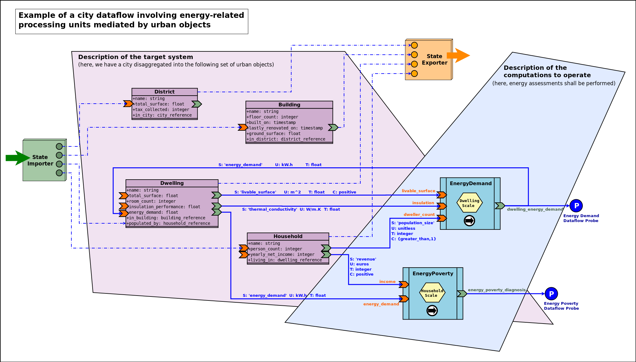
One can also notice:
- two dataflow probes (on the right), should specific results have to be extracted from the dataflow (read here from the output ports of some blocks)
- external state importer and exporter, supposing here that this simulation is integrated into a wider computation chain (respectively in charge of providing an input state of the world at each time step, and, once evaluated and updated by the dataflow, of reading back this state and possibly transferring it to other, third-party, computational components; they are specialised versions of experiment entry and exit points).
We can see that we have still here a rather high-level, abstract view of the dataflow: types are mentioned (e.g. Building) instead of instances (e.g. building_11, building_12, etc.), and managers (discussed later in this document) are omitted.
A View Onto an Actual Simulation
The following instance-level diagram describes the simulation case whose sources are available in the mock-simulators/dataflow-urban-example directory:
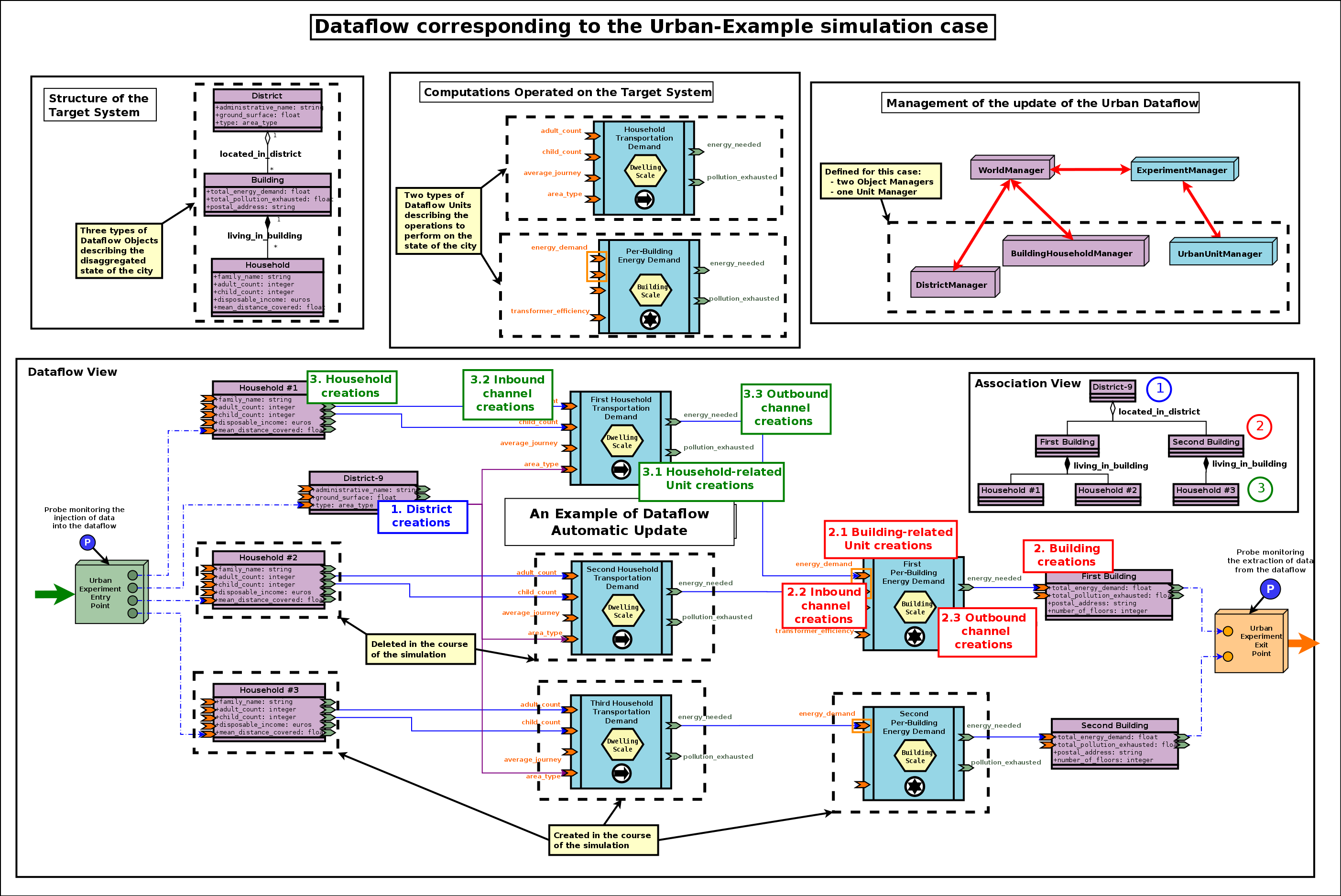
This case demonstrates the following elements:
- two specific entry and exit experiment points
- two types of processing units, one of which relies on an (input) port iteration
- four unit instances
- two unit activation policies
To run that example:
$ cd mock-simulators/dataflow-urban-example/src
$ make batch
Alternatively, to run a display-enabled version thereof, one may run make run instead.
Developing Dataflow Elements in Other Programming Languages
The dataflow infrastructure, like the rest of Sim-Diasca, uses a single implementation language, Erlang, which may be readily used in order to implement, notably, dataflow processing units.
However it may be useful to introduce, in one's simulation, dataflow blocks (e.g. a set of processing units corresponding to at least one model) that are implemented in other programming languages, especially if they are for the most part already developed and complex: integrating them in a dataflow might involve less efforts than redeveloping them.
To ease these integrations, language bindings have been defined, currently for the Python and the Java languages - still to be used from GNU/Linux. These bindings provide APIs in order to develop dataflow constructs in these languages and have them take part to the simulations.
Note that a language binding often induces the use of a specific version of the associated programming language (e.g. the Python binding may target a specific version of Python). We tend to prefer the latest stable versions for these languages (as they are generally more stable and provide more features), however in some cases some helper libraries that might be proposed for inclusion by models (for their internal use) may not be updated yet.
In that case, should these extra dependencies be acknowledged, a language downgrade may be feasible, until these libraries are made compliant again with the current language version.
One should refer to the Sim-Diasca Coupling HOWTO for further information regarding how third-party code can be introduced in a Sim-Diasca simulation, whether or not it is done in a dataflow context.
Python Dataflow Binding
General Information
This binding allows to use the Python programming language, typically to write dataflow processing units.
The Python version 3.6.0 (released on December 23rd, 2016) or more recent is to be used. We recommend to stick to the latest stable one (available here). Let's designate by A.B.C the actual version of Python that is used (e.g. A.B.C=3.6.0).
A Python virtual environment, named sim-diasca-dataflow-env, is provided to ease developments.
Binding Archive
All necessary binding elements (notably the virtual environment and the sources) are provided in a separate archive (which includes notably a full Python install), which bears the same version number as the one of the associated Sim-Diasca install [13].
| [13] | The sources of this binding in the Sim-Diasca repository can be found in sim-diasca/src/core/src/dataflow/bindings/python/src (from now it is called "the binding repository"). |
This binding archive has to be extracted first:
$ tar xvjf Sim-Diasca-x.y.z-dataflow-python-binding.tar.bz2
$ cd Sim-Diasca-x.y.z-dataflow-python-binding
Python Virtual Environment
It should be ensured first that pip (actually pipA.B, like in pip3.6) and virtualenv are installed.
For example, in Arch Linux (as root), supposing that a direct Internet connection available:
$ pacman -Sy python-pip
$ pip install virtualenv
We will make here direct use of the virtual environment that will be obtained next; one may alternatively use virtualenvwrapper for easier operations.
Recommended: Getting this Virtual Environment Directly from the Binding Archive
The virtual environment corresponding to this binding is located at the root of the archive, in the sim-diasca-dataflow-env tree.
It can be used as it is, without further effort.
Alternate Mode of Operation: Recreating this Virtual Environment
If using directly the binding archive is the recommended approach, in some cases one may nevertheless want to recreate the virtual environment by oneself.
Then, as a normal user, an empty environment shall be created, activated and populated with the right packages:
$ virtualenv sim-diasca-dataflow-env --python=pythonA.B
$ source sim-diasca-dataflow-env/bin/activate
$ pip install -r sim-diasca-dataflow-env-requirements.txt
Note
Care must be taken so that the same A.B Python version as the one in the archive is specified here.
We hereby supposed that the Bash shell is used. If csh or fish is used instead, use the activate.csh or activate.fish counterpart scripts.
Using this Virtual Environment
To begin using it, if not already done, one should activate it first:
$ source sim-diasca-dataflow-env/bin/activate
Then all shell commands will use a prompt starting with "(sim-diasca-dataflow-env)" to avoid that the user forgets that this environment is enabled.
Packages provided in this environment shall be managed thanks to pip.
The list of the packages used by default by the binding is maintained in the sim-diasca-dataflow-env-requirements.txt file (available at the root of both the binding archive and repository) [14].
| [14] | It is obtained thanks to: pip freeze > sim-diasca-dataflow-env-requirements.txt. |
From now on, any additional package that one installs (using pip) will be placed in this sim-diasca-dataflow-env directory, in isolation from the global Python installation.
The list of the packages currently used (in the context of this virtual environment) can be obtained thanks to:
$ pip list
Once finished with it, the virtual environment can be deactivated with deactivate (now directly available from the PATH):
$ deactivate
Sources of the Binding
The binding itself, relying for its execution on the aforementioned virtual environment, is a regular (as opposed to a namespace one) Python package named sim_diasca_dataflow_binding, located under the same name at the root of the binding archive [15].
| [15] | As mentioned before, its sources in our repository are located in the sim-diasca/src/core/src/dataflow/bindings/python/src directory. |
Use of the Binding
Let's take the example of a user-defined processing unit, let's say in my_example_unit.py, that may be graphically described as:
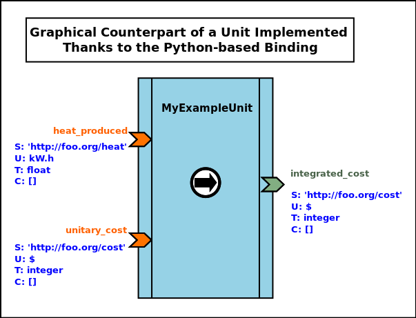
Its corresponding Python-based full implementation may be:
from sim_diasca_dataflow_binding.common import trace
from sim_diasca_dataflow_binding.common import error
from sim_diasca_dataflow_binding.dataflow import unit

class MyExampleUnit(unit.ProcessingUnit):
  """A unit computing heat and fees; 2 input ports, 1 output one."""

  def __init__(self,name:UnitName,relative_fee:float):

    # A static, constant fee applied to some costs:
    self.fixed_fee = 115.0

    # An instance-specific proportional fee:
    self.relative_fee = relative_fee

    my_input_specs = [
      InputPortSpec('heat_produced','http://foo.org/heat','kW.h','float'),
      InputPortSpec('unitary_cost','http://foo.org/cost','$','integer') ]

    my_output_specs = [ OutputPortSpec('integrated_cost',
      'http://foo.org/cost','$','float') ]

    unit.ProcessingUnit.__init__(self,name,my_input_specs,
      my_output_specs,ActivationPolicy.on_new_set)

  def activate(self) -> None:
    """Automatically called by the dataflow, as requested by
       the selected activation policy."""

    input_cost_port='unitary_cost'
    # 'Activate On New Set' policy, hence may be unset:
    if self.is_set(input_cost_port):
      self.debug("Computing fees.")
      cost = self.get_input_port_value(input_cost_port)
      new_cost = self.apply_fees(cost)
      self.set_output_port_value('integrated_cost',
          new_cost)

  # The domain-specific logic is best placed outside of the
  # dataflow logic:
  def apply_fees(self,cost:float) -> float:
    """Applies all fees to specified cost."""

    return self.fee + cost * self.relative_fee
For reference, in sim_diasca_dataflow_binding/dataflow/unit.py, we may have the following definitions (used in our example unit above):
from enum import Enum

# Type aliases (mostly for documentation purposes):

Semantics = str
Unit = str
Type = str
Constraint = str

BlockName = str

PortName = str
InputPortName = PortName
OutputPortName = PortName

PortValue = Any

# Taken from https://docs.python.org/3/library/enum.html#functional-api:
class AutoNumberedEnum(Enum):
   def __new__(cls):
       value = len(cls.__members__) + 1
       obj = object.__new__(cls)
       obj._value_ = value
       return obj


class ActivationPolicy(AutoNumberedEnum):
   on_new_set = ()
   when_all_set = ()
   custom = ()

class InputPortSpec():

  def __init__(self, name:InputPortName, semantics:Semantics,
      unit:Unit, type:Type, constraints=List[Constraint] ):
    [...]


class OutputPortSpec():
    [...]

class Port():
    [...]

class InputPort(Port):
    [...]

class OutputPort(Port):
    [...]


class ProcessingUnit(trace.Emitter):
  """Base, abstract, dataflow processing unit."""

  def __init__(self, name:UnitName, input_specs:List[InputPortSpec],
                  output_specs:List[OutputPortSpec],
                  activation_policy:ActivationPolicy):

    # Class-specific attribute declaration:
    #  - input_ports={} : Mapping[InputPort]
    #  - output_ports={}: Mapping[OutputPort]
    #  - activation_policy: ActivationPolicy

    trace.Emitter.__init__(self,name,category="dataflow.unit")
    self.trace("Being initialised.")
    self.register_input_ports(input_specs)
    self.register_output_ports(output_specs)
    self.activation_policy=validate_activation_policy(activation_policy)

  def register_input_ports(self, specs:List[InputPortSpec]) -> None:
    [...]

  def register_output_ports(self, specs:List[OutputPortSpec]) -> None:
    [...]

  def validate_activation_policy(policy:Any) -> ActivationPolicy:
    [...]

  def is_set(self,name:InputPortName) -> bool:
    """Tells whether specified input port is currently set."""
    [...]

  def get_input_port_value(self,name:InputPortName) -> PortValue:
    """Returns the value to which the specified input port is set.
       Raises ValueNotSetError if the port is not set.
    """
    [...]

  def set_output_port_value(self,name:OutputPortName,PortValue) -> None:
    [...]


  def activate(self) -> None:
    """Evaluates the processing borne by that unit.

    Once a unit gets activated, it is typically expected that it reads
    its (set) input ports and, based on their value and on its own state,
    that it set its output ports accordingly.
    """
    pass
Binding Implementation
The Python dataflow binding relies on ErlPort for its mode of operation.
Please refer to the Sim-Diasca Technical Manual to properly install this binding.
Java Dataflow Binding
This binding allows to use the Java programming language, typically to write dataflow processing units.
The Java version 8 or higher is recommended.
Note
Unlike the Python one, the Java Binding is not ready for use yet.
Other Language Bindings
A low-hanging fruit could be Ruby, whose binding could be provided relatively easily thanks to ErlPort.
Rust could be quite useful to support as well.
More Advanced Dataflow Uses
Dynamic Update of the Dataflow
One may imagine, dynamically (i.e. in the course of the simulation):
- creating or destroying blocks
- creating or destroying channels
- updating the connectivity of channels and blocks
- creating or destroying input or output ports of a block
This would be useful as soon as the target system is itself dynamic in some way (e.g. buildings being created in a city over the years, each building relying on its associated computation units - which thus have to be dynamic as well, at least with varying multiplicities).
Moreover, often all the overall layout cannot be statically defined, and the dataflow as a whole has to be dynamically connected to the components feeding it or waiting for its outputs (e.g. a database reader having to connect in some way to some input ports) - so some amount of flexibility is definitively needed.
Iteration Specification & Iterated Ports
Usage Overview
In some cases, a given type of unit may support instances that can have, each, an arbitrary number of ports relying on identical metadata (i.e. ports that have to obey the exact same specifications).
An example of that is a processing unit aggregating a given metrics associated to each building of a given area: each instance of that unit may have as many input ports (all having then exactly the same metadata) as there are different buildings in its associated area, and the class cannot anticipate the number of such ports that shall exist in its various instances [16].
| [16] | Not to mention that buildings may be created and destroyed in the course of the simulation, so, even for any given instance, the number of ports may have to change over simulation time... |
Supporting iterated ports spares the need of defining many ports that would happen to all obey the same specification; typically, instead of declaring by hand an energy_demand port and similar look-alike ports (that could be named energy_demand_second, energy_demand_third, etc.) with the same settings, an energy_demand(initial,min,max) port iteration can be specified.
This leads, for each instance of this unit, to the creation of initial different iterated ports, all respecting the energy_demand port specification.
At any time, for each of these unit instances, there would be at least min instances of such ports, and no more than max - that can be either a positive integer, a named variable or the * (wildcard) symbol, meaning here that a finite yet unspecified and unbounded number of these ports can exist.
More precisely, in a way relatively similar to the UML conventions regarding multiplicities, for a given port iteration one may specify either a fixed number of iterated ports, or a range:
| Multiplicity | Examples | Meaning: for this iteration, at all times there will be: |
|---|---|---|
| Fixed constant | 7 | Exactly 7 iterated ports |
| Variable name | n | Exactly n iterated ports |
| * | * | Any number of iterated ports |
| Min..Max | 0..4,a..b, 2..* | Between Min and Max iterated ports (bounds included) |
In a given dataflow, variable names (e.g. m, n, o, etc.) are expected to match. For example, if the variable n is referenced more than once in the dataflow, then all its occurrences refer to the same value (which is let unspecified in the diagram).
Iterated ports are automatically named by the runtime (e.g. energy_demand_iterated_1, energy_demand_iterated_2); they are standard ports and thus their name shall remain an identifier [17].
| [17] | This is why the runtime enforces the single restriction that applies to port names, which is that the _iterated_ substring cannot exist in such a user-defined name. |
Graphically, the set of ports corresponding to an iteration is represented as a rectangle enclosing these iterated ports (when representing actual instances, the rectangle may be empty); multiplicities are to be specified between brackets (to distinguish them from the iteration name) and preferably at the bottom of the associated rectangle.
All these elements shall be of the same color as the one of the port. Any common metadata shall preferably be listed once.
An example of these conventions is the following processing unit, featuring two input and and two output port iterations:
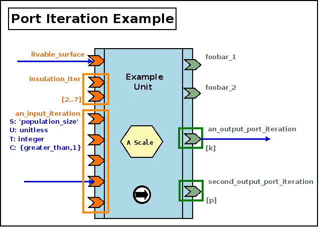
We can see above that, at any time, the first input iteration shall have between 2 and 7 (included) iterated ports, while the second input iterations is detailed graphically and has exactly 5 iterated ports ([5] is thus implied).
As for the output iterations, both have a certain number of iterated ports, and, as k is different from p, their respective counts of iterated ports may not match (e.g. we can have k=2 and p=0).
In Terms of Implementation
An iteration specification enables the creation of multiple (input or output) ports of the same type, each of these instances being designated as an iterated port (technically an iterated port is nothing but a standard port).
For example, defining an iteration specification of 3 instances named foobar will result in the creation of 3 actual (iterated) ports, each complying to this specification, and named foobar_iterated_1, foobar_iterated_2 and foobar_iterated_3 [18].
| [18] | As mentioned, once created, these three ports will be fully standard ports; the _iterated_ substring helps avoiding that the names of iterated ports clash with other ports (it convey no specific meaning as such). |
By default, port specifications are not iterated: in implementation terms, the is_iterated field of a port specification is set to false.
To enable the creation of iterated ports, the is_iteration field of the corresponding port specification shall be set to either of these three forms:
- {Initial,{Min,Max}} where Initial is the initial number of iterated ports to be created according to this specification, and Min and Max are respectively the minimum and maximum counts of corresponding iterated ports that are allowed to exist
- then the runtime will create the corresponding initial number of instances (whose name is suffixed as mentioned with an incremented number starting from 1), and ensure that, even in the presence of runtime port creations, the number of the corresponding iterated ports will remain within specified bounds
- Initial and Min are positive integers, while Max can also be set to the unbounded atom to allow for an unlimited number of such iterated ports; of course Initial must be in the {Min,Max} range
- {Initial,Max}, which is a shorthand of {Initial,{_Min=0,Max}}
- Initial, which is a shorthand of {Initial,{_Min=0,_Max=unbounded}}
Domain-Specific Timestamps
By default, engine ticks directly translate to a real, quantified simulation time: depending on the starting timestamp and on the selected simulation frequency, a given tick corresponds to an exact time and date in the Gregorian calendar (e.g. each month and year lasting for the right number of days - not respectively, for example, 30 and 365, a simplification that is done in some cases in order to remain in a constant time-step setting).
However, in some simulations, models are ruled by such a strange simplified time [19], so domain-specific timestamps may be useful. Their general form is {timescale(),index()}, where timescale() designates the selected time granularity for the underlying channel (e.g. constant_year, month_of_30_days) and index() is a counter (a positive integer corresponding to as many periods of the specified time granularity).
| [19] | Even if this oversimplification just by itself yields already significant relative errors (greater than 10%). |
For example, in a simulation some models may be evaluated at a yearly timescale, while others would be at a daily one. Considering that initial year and day have been set beforehand, a timestamp may become {yearly,5} or {daily,421}. This could be used to check that connected ports have indeed the same temporality (e.g. no yearly port linked to a daily - a timescale convertor unit needing to be inserted in that case), and that none of such timescale-specific timesteps (i.e. index) went amiss in the channel.
Usefulness of Cyclic Dataflows?
One can notice that cyclic dataflow graphs are allowed by this scheme based on input and output ports, and that even "recursive dataflow objects" (i.e. dataflow objects having one of their output port connected to one of their input ones) can exist.
Of course some convergence criterion is needed in order to avoid a never-ending evaluation.
Experiments
As mentioned in the Experiment Definition section, an experiment is the top-level abstraction in charge of driving the computations applying to a simulated world.
Purpose of Experiment Endpoints
Depending on the project, it may be convenient for a given experiment relying on any number of dataflows to define a pair of components in charge of triggering and terminating its evaluation (typically once a specified number of steps were performed), as points of entry and exit, respectively.
For that, base classes are provided (ExperimentEntryPoint and ExperimentExitPoint) that are meant, if needed, to be subclassed on a per-project basis.
The purpose of these (optional) endpoints is to drive multiple dataflow instances, possibly on par with some external software (e.g. any overall integration platform).
Their impact in the progress of an experiment is discussed next.
Experiment Progress
In terms of logical ordering, the usual course of action of a dataflow-oriented simulation discussed here is [20]:
- a new simulation tick T begins: the experiment entry point (which is an actor) is scheduled
- a synchronisation stage, detailed in the next sections, occurs: the dataflows are suspended, and the state of the simulated world is updated first, then the computations that shall be applied on it are modified accordingly
- then the dataflows are resumed, and it usually triggers (based on intermediate logical moments, i.e. diascas) in turn (source) dataflow objects and/or processing units
- this may trigger cascading updates of dataflow elements over diascas
- once all evaluations are done, the experiment exit point (another actor) is to wrap up all information and perform any related tick-termination operation (e.g. sending an update regarding the newer state of the simulated world to a third-party platform)
- then the next planned tick begins (usually this corresponds to T+1), and the process continues until a termination criterion is met (typically a final timestamp is reached, or the simulation is notified that no changes are to be expected anymore)
| [20] | To shed some light on the related implementation (as the technical organisation is a bit different), please refer to the Scheduling Cycle of Experiments. |
As a result, the processing of a given timestep may boil down to an overall three-step process:
- synchronisation of the state of the simulation from an external source (thanks to a state importer - generally an experiment entry point)
- then evaluation of the corresponding dataflow
- then update of an external target, based on the resulting state of the simulation (thanks a state exporter - generally an experiment exit point)
These external source and target may actually correspond to the same data repository, held by a more general platform.
The rest of that HOWTO explained with great detail how step B is tackled. We will thereafter focus thus on step A, knowing that step C in many ways is a reciprocal of this step, and thus may be at least partly deduced from the understanding of step A.
A General View on the Dataflow Synchronisation
The goal is to properly manage the transformation of a source dataflow into a target one, in the context of the simulation of a system.
More precisely, here the source dataflow is the one obtained after the evaluation of a timestep, while the target dataflow is the one that shall be evaluated at the next timestep.
In-between, an external operator may apply any kind of changes to the simulated system, and of course these changes shall be reflected onto its dataflow counterpart.
Such changes may be defined programmatically [21] or be discovered at runtime from an external source [22]. The next sections will focus on the latter case, which is the trickier to handle.
| [21] | If the dataflow is to be managed programmatically (i.e. thanks to specific code), then a user-defined program is to use the various dataflow-relative primitives in order to create the initial state of the dataflow and possibly update it in the course of the simulation; see, in mock-simulators/dataflow-urban-example, the dataflow_urban_example_programmatic_case.erl test case for that. |
| [22] | This setting is illustrated by the dataflow_urban_example_platform_emulating_case.erl test case. |
As already mentioned, dataflows are made of blocks, linked by channels, and two different sorts of blocks exists here:
- the dataflow blocks, which are in charge of describing the current state of the simulated world
- the dataflow processing units, which are in charge of performing domain-specific computations onto that state
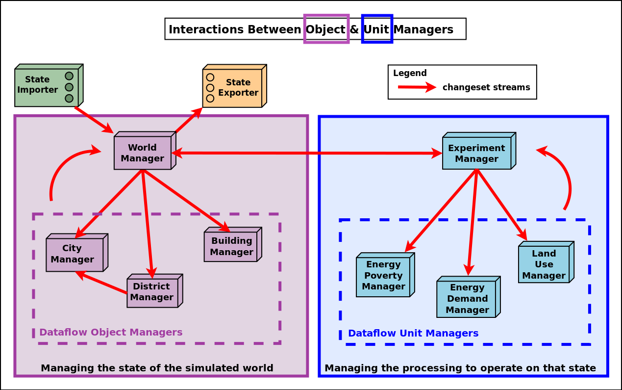
Let's introduce first, and in a few words only, the main elements that are provided in order to transform a dataflow into another:
- the changes in the state of the simulated world are orchestrated by the World Manager, driving the various Object Managers for that
- the changes in the computations to be operated are orchestrated by the Experiment Manager, driving the various Unit Managers for that
- each change is described by an individual World Synchronisation Event, meant to affect potentially both the state of the simulated world and, in turn, the computations operated on it
- a Changeset may aggregate many of these events, and a dataflow can be turned into another by simply applying a series of changesets
The diagram below gives a synthetic, example view of the overall mode of operation in action:
Let's discuss now more precisely the various elements of the solution, and how they interact.
The World Manager and its Dataflow Object Managers
Purpose of the World Manager
This manager (singleton instance of the WorldManager class), whose shorthand is WM, is used in order to create, update and keep track of the simulated world and its structure; this world is itself made of the target system of interest (e.g. a city) and of its context (e.g. its associated weather system, the other cities in the vicinity, etc.).
As a result, the world manager is generic, yet its use is specific to a given modelling structure (e.g. to some way of describing a city), and bears no direct relationship with the computations that will be performed on it (one of its purposes is indeed to help uncoupling the description of the world of interest from the models operating on it, so that they can themselves be defined independently, one from another).
This virtual world is to be modelled based on various types of dataflow objects. For example, if the target system is a city, then districts, roads, buildings, weather elements, other cities, etc. may be defined (as types first, before planning their instantiaton) in order to represent the whole.
These dataflow objects, which account for the state of the simulation world, are to be defined individually (in terms of internal state; e.g. a building has a surface and an height attributes, of corresponding SUTC metadata) and collectively (in terms of structure and relationships; e.g. a building must be included in a district, and may comprise any number of dwellings).
Purpose of the Object Managers
For each of these types of dataflow objects, an object manager, in charge of taking care of the corresponding dataflow objects (i.e. the instances of that type) must be defined [23]. For example the BuildingManager will take care of (all) Building instances.
Note that a given object manager is to take care of at least one type of objects, possibly multiple ones (e.g. if deemed more appropriate, a single object manager may be defined in order to take care of the buildings and of the households and and the districts).
| [23] | All actual dataflow managers are either instances of the DataflowObjectManager class (for the simpler cases), or child classes thereof (e.g. to support specifically some kind of associations). All these managers are themselves simulation actors, as interacting with them in the course of the simulation may be necessary (e.g. to create new object instances). |
The purpose of an object manager is to be the entry point whenever having to perform dataflow-level operations on the object instances of the type(s) it is in charge of (e.g. actual buildings): in the course of the simulation, instances may indeed have to be properly created, associated, connected, modified, deleted, etc.
Finally, all dataflow object managers are federated by this WM (World Manager), which is their direct parent, in charge of driving them all.
The main use of the world manager and of its associated dataflow object managers is the enabling of external state synchronization.
Should, for example, an overall, targeted simulation be actually performed by a pipe-line of platforms (including of course at least the one at hand, which is based on this dataflow infrastructure), at each time step the state of the simulation would need to be updated from these other platforms and, reciprocally, once modified by the dataflow-based one, would need to be passed to the next platforms.
The various dataflow objects involved in the simulation have to reflect the current state of the world; for that, from one timestep to the next, changes have to be applied onto them. For example, if the evaluation runs on a yearly timestep, handling simulation year 2026 requires that changes that happened since the end of the dataflow evaluation of 2025 are taken into account before starting to simulate year 2026.
Expressing Dataflow Changes Through World Events
These changes are expressed at the dataflow level thanks to world (synchronisation) events. Following types of world events [24] have been defined:
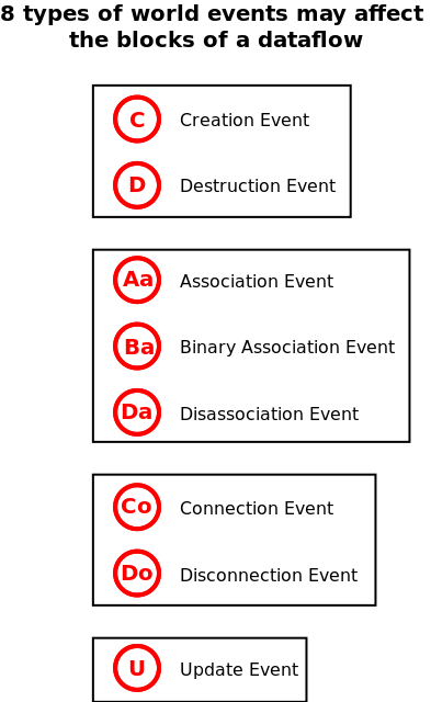
| [24] | Refer to dataflow_changesets_defines.hrl for their actual definitions: for each type of event, a corresponding datastructure is defined in order to store the identifier of each event, the type of dataflow object it refers to, the external and internal identifier of the instance(s) involved, extra type-specific information, etc. |
More precisely:
- a creation event describes the creation of a block, typically of a dataflow object (e.g. building B2 being built in the city on the current year)
- a deletion event describes the deletion of a block, typically of a dataflow object (e.g. district D7 being destructed)
- an association event describes the creation of an association between dataflow objects; a binary association is a very common, special case thereof (e.g. building B2 is "located in" neighborhood N3)
- a disassociation event describes the removal of an association between dataflow objects (e.g. household H1 is not "living in" building B2 anymore)
- a connection event describes the creation of a dataflow channel between two ports of blocks, from an output one to an input one (e.g. from the surface output port of building B6, to the average_area input port of the land-use processing unit L9)
- a disconnection event describes the deletion of a dataflow channel that used to exist between two ports
- an update event describes the modification of the value of attributes of a dataflow object (e.g. for building B2, the surface attribute is set to 120.0 m^2, while its inhabitant_count is set to 7)
Should, for a given project, the incoming dataflow updates deal only with the state of the simulated world (not directly with the computations themselves - whose changes may be automatically deduced from the state ones at a latter step), only a subset of the types of world events are to be supported (by the world manager), namely all types of events but connections and disconnections.
Changetrees and Changesets
A given event may induce any number of other events (e.g. a creation of a building may induce its association with a given district), which themselves may induce in turn other events, and so on.
As a result, we define the concept of changetree (an event and all the ones it induces, directly or not) and of changeset (a list of changetrees):
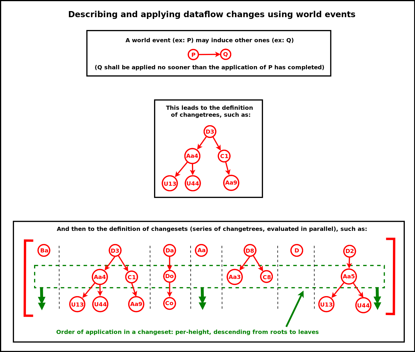
It is the role of the dataflow entry point (typically fetching its informations from an external source) to stream the corresponding changesets to the world manager, and to notify it when the synchronisation has been fully described (i.e. when all changesets have been transmitted).
Changeset Crunching
When the world manager receives a changeset, it dispatches each event in turn to the relevant object manager, based on the type of the dataflow object to which this event applies. For example an event about the creation of a building will be transmitted to the object manager which declared it was in charge of the dataflow objects of type Building.
Events are processed by the world manager based on their height on the pending changetrees, so that their order of induction is preserved : first the root events of all changetrees of the current changeset are dispatched (in an asynchronous way, all in parallel, during the same logical moment), then, when one of these events is reported (by the corresponding object manager) as completed, the world manager dispatches in turn the events that it is inducing, and so on (as a result, if event E1 induces event E2, the processing of E2 will not start before the completion of the processing of E1 [25]). All the changetrees progress in parallel, and each at its maximum rate (knowing that not all operations triggered require the same number of diascas to complete).
| [25] | This is a necessary feature; for example, if E1 is a creation of a building and E2 is its association, E2 will need to rely on an already fully created object before being able to define any association involving it. |
Moreover, when an object manager reports to the world manager the completion of event(s), it may as well inject new events. For example, if creating a building entails creating three lifts, then the building object manager may inject three additional lift creation events. Then these events will be processed, among the pending others, by the world manager, and thus will be dispatched to the lift object manager. This allows for an indirect communication between object managers, and to embed, if needed, domain-specific rules in order to structure appropriately the state of the simulated system.
Note
During the whole synchronisation phase, the blocks of the dataflow that are affected (e.g. created or updated) are put in stasis, i.e. they are suspended.
Otherwise their evaluation could start whereas the dataflow did not reach yet a stable state, which could lead to an incorrect evaluation of the overall dataflow.
To anticipate a bit, the actual evaluation will take place when the dataflow(s) will resume their suspended blocks, which will happen later - once the experiment manager will have finished its own synchronisation work.
As changesets are streamed and processed, the world manager collects the completed events, in a flat, ordered list: all events are enumerated there according to their processing/induction order (i.e. if E2 is induced by E1, E1 will be listed before E2), and they will not embed induced events anymore (so that each event is present exactly once in this flattened list).
Once in a final state (all changesets transmitted and processed), the corresponding overall aggregated completed changeset is sent to the next stage of the dataflow update, dealing this time with the computational part thereof - as explained in the next section.
The Experiment Manager and its Unit Managers
Purpose of the Experiment Manager
The Experiment Manager is a component (singleton instance of the ExperimentManager class), whose shorthand is EM, and that is responsible for the management of the processing part of the dataflow(s), i.e. of the computations that are to be operated on the simulated world, accounting for the experiment that is to take place onto the simulated world.
These (model-specific) computations are implemented by processing units, which are driven by the unit managers - which are themselves federated by the experiment manager.
As a result, the experiment manager is generic (while its use is domain-specific), and it can be seen as an orthogonal counterpart of the world manager, according to this table matching concepts:
| State of the Simulated World | Computations to be Operated |
|---|---|
| Dataflow Object | Dataflow Processing Unit |
| Object Manager | Unit Manager |
| World Manager | Experiment Manager |
Having them separated allows to isolate and uncouple more easily the operations to be performed from the elements they are to operate on. They however both rely on changesets to perform their operations.
Purpose of the Unit Managers
Dataflows may rely on any number of unit managers.
A Unit Manager is in charge of taking care of all instances of at least one type of units involved in the dataflow [26], for a given model; as such, a unit manager may typically create, delete, modify (including reconnecting) the units of the type(s) it supports.
| [26] | All actual unit managers are child classes of the UnitManager base class, to handle the operations specific to the types of the processing units that they support. |
Let's say for example that, for a given model, we have, among other ones, two types of processing units, EnergyDemandUnit and WaterDemandUnit that are to operate each on a given building.
A unit manager named ResourceDemandUnitManager may be in charge of all instances of these two types of units, for example so that it can be ensured that the two kinds of demands are appropriately interlinked and applied consistently (e.g. exactly to the same buildings).
Note
Most models rely on multiple types of processing units - yet on a single, unified unit manager instance that drives them all.
However one can instead define, for a given model, multiple unit managers, each in charge of a subset of the types of processing units involved - provided that these unit managers partition these unit types, i.e. that each unit type is driven by exactly one unit manager instance.
If such a scheme allows the work on the processing units to be split in more autonomous parts, it induces limitations: relying on a single unit manager allows to store in its state all unified information about dataflow objects (based on the world events it listens to) and units (as, for that model, it is their sole manager), which is often necessary to perform proper channel creations (e.g. to determine the right instance of processing unit to be connected to a given dataflow object).
As a result, unit managers tend to define various associative tables, to keep track of which processing unit they created (e.g. a pollution computation) in response to the creation of which dataflow object (e.g. a car). Unit managers are then able to connect these units adequately, once they are reported as created.
As a result, each unit manager federates the units of specific types, so that it can perform - for computations and on behalf of the EM - what dataflow object managers perform for the simulated world on behalf of the WM [27]: a unit manager will synchronise the computation part of the dataflow regarding these unit types.
| [27] | Similarly to object managers, unit managers typically take part to the simulation (e.g. they may create processing units) and therefore must be properly synchronized; as such they are simulation actors as well. |
Mode of Operation
This synchronisation of the computational part of the dataflow could be explicitly dictated by an external source, as done previously for the part of the dataflow devoted to the description of the state of the simulated system. However, more often than not, the changes in the computation part may be determined automatically from the changes done on the state part, based on relevant rules. The purpose of the unit managers is to implement said rules.
To do so, each unit manager is to declare not only the types of processing units it is to manage (e.g. ResourceDemandUnitManager taking care of EnergyDemandUnit and WaterDemandUnit), but also the world synchronisation events it listens to, and how it is to react to them.
For example, ResourceDemandUnitManager may request to be notified whenever a building is created and/or whenever the current operating state of a given heat pump changed (e.g. from nominal mode to degraded mode). It may then choose to apply the relevant domain-specific actions in order to adapt the computations performed by the dataflow, such as, respectively, creating one instance of EnergyDemandUnit and of WaterDemandUnit and connecting them to the new building, or linking said heat pump to a different processing unit implementing a model corresponding to its new mode of operation (by updating their dataflow connectivity).
In practice, a given unit manager may declare (to the experiment manager) any number of event match clauses [28], whose granularity can be finely tuned (from a non-discriminating unit manager listening to all events of all types, to one focusing only on very precise matches [29]).
| [28] | Refer to dataflow_changesets_defines.hrl for their actual definitions: for each type of event match (e.g. creation_event_match), a corresponding datastructure is defined in order to store against which element(s) of the corresponding event the match shall be done (e.g. "the (created) object type shall be of type Building, it should occur in the context of this dataflow, involve a dataflow object bearing this external identifier and/or this internal one, specify these construction parameters, etc.). |
| [29] | Of course a unit manager is free to perform any additional, arbitrary filtering it may need, simply by ignoring the notified events that would not be deemed of interest. |
Then, when the World Manager will transmit the aggregated changeset [30] to the Experiment Manager, this latter simulation agent will iterate through the events in turn, and notify the unit managers whose event clauses matched [31].
| [30] | A single, aggregated changeset is relied upon on purpose: if changesets were streamed by the World Manager to the Experiment Manager as they complete, unit managers would have to be able to operate on an unstable dataflow view of the system state (i.e. subject to changes due to further changesets), which could jeopardize the correctness of the synchronisation of the computational part. |
| [31] | Translating to calling their appropriate event handler; for example, should a given event match a binary_association_event_match declared by a unit manager, the experiment manager will transmit this event to this unit manager, by calling its onBinaryAssociationEventMatched method. |
This unit manager will then be free to react appropriately to this listened event, by performing changes onto the computational part of the underlying dataflow. As hinted in the ResourceDemandUnitManager example, typical changes are to create or delete a processing unit, or to connect or disconnect ports of a processing unit to ports of dataflow objects [32].
| [32] | As a result, unit managers have to rely on a corresponding API, possibly implemented also in the language bindings. For example, a Python-based unit manager would use methods inherited from the UnitManager base class, such as the self-explanatory create_unit or connect_unit methods. |
About Mock-up Units
Mock-up units are units that, instead of implementing a computation logic, directly compose the state of their output ports based on the one of their input ports, relying for that on the static information (data, not code) that they embed.
As such, mock-up units merely associate pre-recorded outputs to inputs, instead of implementing computations allowing to determine the former from the latter ones.
These mock-up units can act as "termination plugs", i.e. placeholders inserted in a dataflow in order for example:
to replace an actual unit (e.g. to wait until it is delivered)
to emulate the context of another unit in order to better test it
to validate an implemented unit against reference input/output datasets
to provide a simpler, less computation-demanding version of a unit (see model order reduction, called metamodel in some communities)
In practice, these mock-up units are instances of the DataflowMockupUnit class (or of a child class thereof), which provides a generic mock-up unit able to be fed with data basically describing, in terms of ports, which outputs are to correspond to which inputs.
They are instantiated and managed by a unit manager, just like any processing unit would do. The only difference is that, since their construction parameters are slightly different from classical units, they have to be created by dedicated methods that have been added to the DataflowUnitManager class.
Definition of a Mock-up Unit
A mock-up unit is specified exactly as any other dataflow unit (e.g. with a name, a temporality, a description of its input and output ports), yet it has to replace the inner computation logic that would be included in any standard unit by a (static) association determining its outputs from its inputs.
This association can be seen as a simple function which, based on a given (optional) simulation time and an input match specification operating on its input ports, tells in which state the output ports of this mock-up unit shall be.
One should note that the result returned by this function (the actual state of the output ports) will depend only on its input parameters (the specified time and the input match specs); for example no contextual data can intervene, because this (pure) function is stateless (i.e. it has no memory).
The general form of this mock-up function is:
f(time(), input_match_spec()) -> output_state()
This means that the purpose of this mock-up function is to tell, for a given simulation time and for a configuration of the input ports that matches the supplied specification, what is the corresponding updated state of at least some of the output ports of that unit.
Multiple clauses can be specified in order to fully define that function: at runtime, at each activation, each of these clauses will have its time and input specifications matched against the current simulation time and the state of the input ports. The first clause to match will be the only one executed during this activation, leading to applying the state changes on the output ports that it specifies. Should no clause match, the mock-up unit will simply stay inactive until the next activation (no specific signal will be sent to the downstream connected blocks).
Examples in the next sections will clarify this mode of operation; let's call from now the mock-up function f/2, i.e. a function named f taking two parameters, respectively the time and the input match spec.
Simulation Time Specification
A mock-up function may react differently at different time steps of the simulation. So a clause of that function may specify, for its first parameter:
- either the precise time step at which it shall be applied, for example f(127,...)->..., to denote here that this clause corresponds to the simulation step #127
- or the any_time atom, to tell that the application of this clause does not depend on simulation time; as a result, f(any_time,...)->... will match irrespectively of the current time step
Of course units (hence mock-up ones) may be atemporal, in which case only timeless clauses (using any_time) would be used.
Input Match Specification
This second parameter of the mock-up function allows to specify the configuration of input ports to which this clause is meant to match: the match specification describes the possible states in which the input ports of interest for the mock-up unit shall be, for this clause to be selected. That clause determines in turn the state of the output ports that will be consequently retained.
In practice, an input match spec is an (unordered) list of pairs, whose first element designates an input port, and whose second one specifies the associated state(s) that would match.
This first element is the name of the input port (e.g. "I1"), as, in the context of a unit, it is an identifier (it is unique).
The second element of the pair associated to a listed input port is among:
- the any_state atom, to specify that the state of this input port will be ignored, i.e. that it may or may not be set (if set, its value will not matter for the clause)
- the unset atom, to specify that this input port should not be set
- the set atom, telling that this input port may have any value, provided it is set at all
- a {set,V} pair, requiring that input port to be set exactly to this value V
- a {between,A,B} pair, requiring that input port to be set to a scalar, numerical value in the [A,B] range (hence including bounds)
- a {around,V,E} pair, requiring that input port to be set to a value around V, with a relative error [33] of up to E; this is a way of better supporting floating-point values - for which strict equality is usually not meaningful
- a {around,V} pair, requiring that input port to be set to a value around V with a default relative error of 1.0e-6
- a {among,[V1,V2,..,Vn]} pair, this input port having to be set to one value in that list for the clause to possibly match
| [33] | The relative error between X and Y being the absolute value of their difference divided by their average value: 2*abs((X-Y)/(X+Y))), for X different from -Y (otherwise abs(X-Y) is used instead). |
Any input port that is not listed in the spec may be in any state (unset, or set to any value); the any_state atom is therefore a way of specifying the same, yet in an explicit manner.
For example, if a unit has six input ports named "I1", "I2", "I3", "I4", "I5" and "I6" [34], and the input match specification is:
[{"I2", {set, 14.0}}, {"I5", set}, {"I4", {between, {2,8}}},
  {"I1", unset}, {"I6", {among, [3,4,6]}}]
| [34] | Please note that the coupling layer allows port names to be any string; input ports do not have to be named "I1", "I2", etc.; therefore "attila woz here" and "FelixTheCat-1337" would be perfectly suitable (and of course the same applies to the name of output ports as well). |
Then this function will match iff (if and only if), in terms of input ports for that mock-up unit:
- "I1" is unset (i.e. not set to any value)
- and "I2" is (exactly) set to 14.00
- and "I4" is set to a value in [2,8]
- and "I5" is set (to any value)
- and "I6" is set to 3, 4 or 6
One can note that the order of the pairs does not matter, and that the input port "I3", not being listed, can thus be in strictly any state.
Output State Specification
When a given clause is evaluated (implying none of the previous ones could apply), if both its current time and input specifications are matching the current runtime and state information, then this clause is selected, and the output ports of the mock-up unit are then set as this clause specifies.
An output state is defined as an (unordered) list of pairs, whose first element designates an output port (identified by its name), and whose second one specifies the associated state it should be set to.
Possible specified states are:
- the reassign atom to set again this port to the same state, whatever it is
- the unset atom, so that the corresponding output port is (becomes or remains) explicitly not set
- a {set,V} pair, where V is the value to which this output port shall be set
- a {state_of,I} pair, where I is the name of an input port of that unit, in which case the state of the output port will be assigned to the one of the specified input port
If an output port is not listed in the specification, then it will be kept in its current state, knowing that all output ports are initially, once created, unset.
The reassign atom is therefore a way to feed again the connected channel with the same value as it held previously. If this port was previously unset, it will simply stay so.
Knowing that the setting of an output port is punctual (i.e. a one-time event is sent, then the output port comes back to its unset base state), we can see that, in a clause, an output port can be considered as always being initially unset. As a consequence, specifying the unset atom for its new status is optional (since not specifying at all that output port does the same).
For example, if the output state specification of a clause is:
[ {"O7", reassign}, {"O1", {set,6}},
  {"O2", {set,3.14}}, {"O5", {state_of,"I2"}} ]
then, should this clause be selected, the output ports of this mock-up unit will be assigned to the following state:
- "O1" set to 6
- "O2" set to 3.14
- "O5" having the same state as input port "I2"
- "O7" staying unchanged
- all other ports being inactive (as if they were unset)
Consistency and Checking
Of course, both the input match specifications and the output state specifications must respect the typing information (the T in SUTC) of the ports that they may reference.
For example:
- {between,1.1,1.7} cannot apply to an input port typed as a boolean one
- {state_of,I} should not be specified if the corresponding output port has not the same associated type information as the input port I
The dataflow infrastructure will perform some basic checking at runtime, yet some care should be taken by the user to inject only legit data.
Examples of a Mock-up Function
Now such a definition should be quite easy to interpret:
f( 0, [ {"ip_1", {set,true}}, {"ip_3", {set,3}} ] ) ->
   [ {"op_2", {set,89}}, {"op_4", {set,false}} ];

f( 0, [] ) ->
   [ {"op_1", {set,1}}, {"op_2",unset} ];

f( 1, []) ->
   [ {"op_2", {state_of, "ip_7"}} ];

f( any_time, [] ) ->
   [ {"op_4", {set,true}} ].
Indeed that mock-up function f is defined thanks to four clauses, to be read as detailed below.
The first clause will require, if at time step 0, an exact match for both the input ports named "ip_1" (which must be set to true) and "ip_3" (which must be set to 3). If this occurs, then the evaluation of f is over and output ports "op_2" and "op_4" will be set respectively to 89 and false, while the other ones will be unchanged.
Should this first clause not match, the second one will be tried. It references the same time step 0, yet has an empty input match spec. This means that, for that time step, it will be a "catch-all" clause, i.e. a clause that will match necessarily, regardless of the state of the input ports. In this case "op_1" will be set to 1, "op_2" will be explicitly unset, and the state of the other output ports will remain as it is.
As the third clause deals with another time step than 0, it has a chance to match (the previous clauses covered all possible cases for time step 0). We see that it behaves as a catch-all for time step 1, resulting in the "op_2" output port having the same state as the "ip_7" input port.
Finally, the fourth clause is an universal catch-all, for all time steps and all configurations of input ports. This implies that the corresponding mock-up unit will be able to be evaluated in all possible cases; the role of this particular clause here is only to set the "op_4" output port to true.
Another example is a very simple one, the universally defined identity mock-up function, defined as:
f(any_time,[]) ->
 [].
Data-Based Mock-up Definition
A mock-up unit can be seen more as data (output sets being matched to input ones) than as code.
Therefore, rather than implementing a mock-up function as done in the previous section, a means is provided in order to define such a function based on an information stream (typically a file).
Defining the syntax of these data is the purpose of our Dataflow Unit Mockup Format (abbreviated as DUMF), described here. As a consequence, we recommend that the file extension for such a content is dumf, like in: my_model_v4.dumf.
Fortunately, the corresponding data-based descriptions are directly similar to the implementations that have been detailed above:
- a mock-up function was implemented as a series of clauses, its data counterpart is an (ordered) list of clause definitions
- each implemented clause of that function corresponds then to an item of that list, i.e. a clause definition made of two elements:
- the first element is a pair defining the time information and input match specification corresponding to this clause
- the second element details the output state definition that will be applied, should the first element match
So the full, data-based version of a unit relying on the same clauses as specified in the first mock-up function example section may simply be a my_mockup_example.dumf file whose content may read as (note the few ellipses done with "...", in order to shorten the listing):
% This DUMF data file defines the mock-up version of the
% 'class_MyExampleUnit' unit.

% First the metadata for this unit:
{ unit_type, 'class_MyExampleUnit' }.
{ mockup_author, "Jiminy Cricket" }.
{ mockup_author_contact, "jc@fantasy-world.org" }.
{ mockup_version, "1.0.3" }.
{ mockup_date, "16/2/2017" }.
{ activation_policy, activate_when_all_set }.

% Then the definition of its input ports:
{ input_port_specs, [
   [   { input_port_name, "ip_1" },
       { value_semantics, 'http://foo.org/energy' },
       { value_unit, "kW.h" },
       { value_type_description, "float" },
       { value_constraints, [ positive ] } ],
   [   { input_port_name, "ip_2" }, ... ],
   [   { input_port_name, "ip_3" }, ... ],
   ... ] }.

% Followed by the definition of its output ports:
{ output_port_specs, [
   [   { output_port_name, "op_1" }, ... ],
   [   { output_port_name, "op_2" }, ... ],
   ... ] }.

% Finally we define in which state the output ports of this unit
% shall be, based on the following input match specs:
{ mockup_clauses, [
   { {0,[{"ip_1",{set,true}},{"ip_3",{set,3}}]},
        [{"op_2",89},{"op_4",false}]},
   { {0,[]},
        [{"op_1",1},{"op_2",unset}]},
   { {1,[]},
       [{"op_2",{state_of,"ip_7"}}]},
   { {any_time,[]},
       [{"op_4",true}]}
 ] }.

% End of the mock-up definition.
These two forms (these mockup_clauses and the previous function f/2) are basically the same.
As a result, this DUMF file fully describes a mock-up unit that may be represented as:
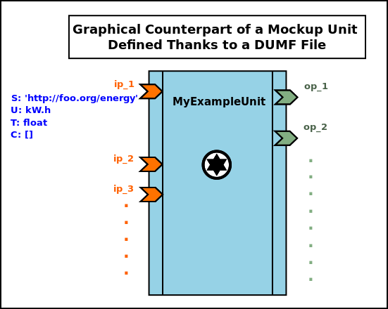
Once the clauses are expressed according to this format, one may think of creating mock-up units directly from such a stream of information, without writing any code.
For that, the DUMF format includes not only these clauses, but also all the other informations that a mock-up unit - as any other processing unit - must provide. Namely:
- metadata such as its name, the type of this unit (e.g. of use for its (unit) manager), etc.
- the specification of its input and output ports
These three blocks of data, with the final addition of the clauses, form a complete description of a mock-up unit, and thus an operational DUMF stream.
See below an example of conforming file, ReferenceExampleMockup.dumf:
% This DUMF data file defines the mock-up version of the unit named:
% class_MyExampleUnit
%
%
% Please refer to the 'Sim-Diasca Dataflow HOWTO' for more information
% about Mock-up Units.
%
% Generated on 21/03/2017 18:04:31, by user 'jiminy'.
%

{ dumf_version, "0.3.1" }.

{ unit_type, 'class_MyExampleUnit' }.

{ mockup_author, "Jiminy Cricket" }.
{ mockup_author_contact, "jc@fantasy-world.org" }.

{ mockup_version, "1.0.0" }.
{ mockup_date, "16/02/2017" }.

{ activation_policy, 'activate_when_all_set' }.


{ input_port_specs, [

    [
        { input_port_name, "ip_1" },
        { comment, "This is my first input port" },
        { is_iteration, 'false' },
        { value_semantics, 'http://foo.org/energy' },
        { value_unit, "kW.h" },
        { value_type_description, "integer" },
        { value_constraints, [positive] }
    ],

    [
        { input_port_name, "ip_2" },
        { comment, "This is my second input port" },
        { is_iteration, 'false' },
        { value_semantics, 'http://foo.org/pollution' },
        { value_unit, "g.cm^-3" },
        { value_type_description, "float" },
        { value_constraints, [] }
    ],

    [
        { input_port_name, "ip_3" },
        { comment, "This is my third input port" },
        { is_iteration, 'true' },
        { value_semantics, 'http://foo.org/length' },
        { value_unit, "m" },
        { value_type_description, "integer" },
        { value_constraints, [non_null] }
    ]

] }.


{ output_port_specs, [

    [
        { output_port_name, "op_1" },
        { comment, "This is my first output port" },
        { is_iteration, 'false' },
        { value_semantics, 'http://foo.org/adult_count' },
        { value_unit, "dimensionless" },
        { value_type_description, "integer" },
        { value_constraints, [positive] }
    ],

    [
        { output_port_name, "op_2" },
        { comment, "This is my second output port" },
        { is_iteration, 'true' },
        { value_semantics, 'http://foo.org/operation_status' },
        { value_unit, "dimensionless" },
        { value_type_description, "boolean" },
        { value_constraints, [] }
    ],

    [
        { output_port_name, "op_3" },
        { comment, "This is my third output port" },
        { is_iteration, 'false' },
        { value_semantics, 'http://foo.org/operation_status' },
        { value_unit, "dimensionless" },
        { value_type_description, "boolean" },
        { value_constraints, [] }
    ],

    [
        { output_port_name, "op_4" },
        { comment, "This is my fourth output port" },
        { is_iteration, 'false' },
        { value_semantics, 'http://foo.org/pollution' },
        { value_unit, "g.cm^-3" },
        { value_type_description, "float" },
        { value_constraints, [] }
    ]

] }.


{ mockup_clauses, [

  { 0,
    [
        { "ip_1", { between, 2, 5 } },
        { "ip_3", { set, 3 } }
    ],
    [
        { "op_2", { set, false } },
        { "op_4", { set, 89.5 } }
    ] },

  { 0,
    [
        { "ip_2", { around, 42.0, 0.0001 } }
    ],
    [
        { "op_1", { set, 1 } },
        { "op_2", unset }
    ] },

  { 1,
    [
        { "ip_3", { among, [1,2,3] } }
    ],
    [
        { "op_4",
          { state_of, "ip_2" } }
    ] },

  { any_time,
    [
        { "ip_1", unset }
    ],
    [
        { "op_2", { set, true } }
    ] }

] }.
Such a complete description of a mock-up may simply be stored in a file, so that it can be later re-used through the read_mockup_unit_spec/1 static method of the DataflowMockupUnit class, allowing a unit manager to create instances of this mock-up unit, for example thanks to the create_initial_mockup_units/4 static method of the DataflowUnitManager class.
The concept of mock-up variety is currently purely documentary. Mock-up units are classical processing units to which we attach a set of mock-up clauses (in order to define their behaviour when activated). Thus, it is possible to imagine having two mock-up units sharing all the attributes of a processing unit but acting according to different mock-up clauses: we would then distinguish them as two varieties of a same mock-up unit type [35].
| [35] | This vocabulary distinction appears from the fact that we are concerned with emulated models, and each emulated model corresponds to an emulated (mock-up) unit_type in the DUMF specifications (since even more generally in dataflows, with the vocabulary of Sim-Diasca, a model is implemented as a type of processing unit). If we imagine a mock-up designer defining two different sets of clauses in two DUMF files which declare a same unit_type (and share the same values for everything else but the clauses), then we end up with two varieties of this same emulated model (or varieties of this mock-up unit type). If it is not clear enough, we can put it in other words: since a fixed set of clauses leads to instantiate identical mock-up units (a variety), we can instantiate a different kind of mock-up units by just modifying the clauses (then creating other varieties). |
About naming the DUMF file, the basic convention is that if one wants to make a mock-up unit emulating a future real model, say a Python unit that would be named VehicleTypeUnit and which would be implemented in vehicle_type_unit.py for instance, then it should be done in a file named VehicleTypeMockup.dumf.
Of course, in practice, the DUMF format is most probably too low-level, too textual for domain experts or model implementers to make a direct use of it.
Indeed units can easily have several dozens of input and output ports, and mock-up units may have to be defined over a very large number of time steps.
Two approaches were then imagined to ultimately obtain the mock-up data in that targeted format:
- defining a lightweight GUI in order to ease (and check) the entering of these information, storing them in this mock-up format
- defining a spreadsheet-based template that would be filled by the persons closer to the models and then automatically translated into a proper mock-up data-based definition
- such a template, compliant with LibreOffice and Microsoft Office, has been devised in order to streamline the specification of mock-up units
- the filled templates (saved as OpenDocument file, whose extension is *.ods) can then be automatically translated into their canonical DUMF counterpart (see our spreadsheet-to-dumf.escript script for that)
While such a GUI is not implemented yet, it is now possible to write a mock-up definition in a spreadsheet and to convert it in the DUMF format seen above.
Mock-up Definition from a Spreadsheet
The script translating a user-defined spreadsheet to a DUMF file needs the former to stick to a template, which is also provided in the Sim-Diasca repository.
The template spreadsheet was first designed using Microsoft Excel 2013 and is named MockupReferenceExample.xlsx. We exported it to the ODF format used for instance by LibreOffice 5, resulting in MockupReferenceExample.ods [36].
Both formats are supported by the script.
| [36] | The path to all the mock-up support in Sim-Diasca is sim-diasca/src/core/src/dataflow/mockup_support. The transformation script can be found there, named mockup_spreadsheet_to_dumf.escript and the template spreadsheets are in the tests subdirectory (alongside the previous example of DUMF file). |
One may note that, for general clarity, the previous naming convention should still hold, by simply adapting the file extensions. Hence for a target model VehicleTypeUnit, the Excel version of the mock-up definition file should be VehicleTypeMockup.xlsx and the ODF version should be VehicleTypeMockup.ods.
Here is the reference Excel spreadsheet cited above, consisting of four worksheets, each representing one of the four blocks of data seen in the previous DUMF example [37].
| [37] | The overall structure of ReferenceExampleMockup.xlsx, as well as the structures of the individual worksheets, are protected by a password. Currently, this password is dataflow. |
First, the metadata associated to a mock-up unit:
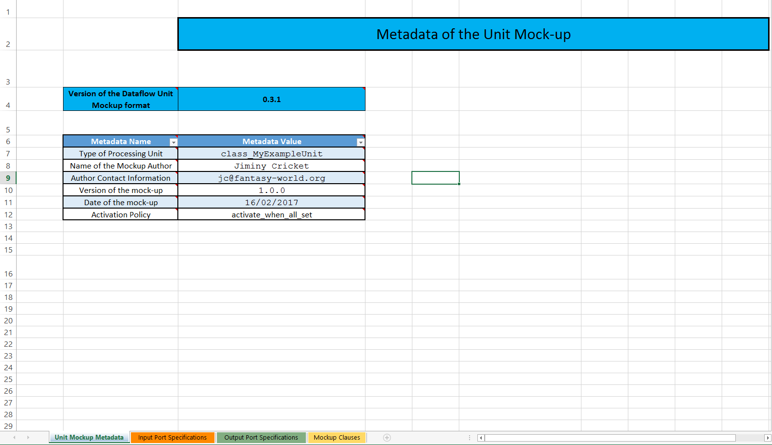
Second, the definition of its input ports:
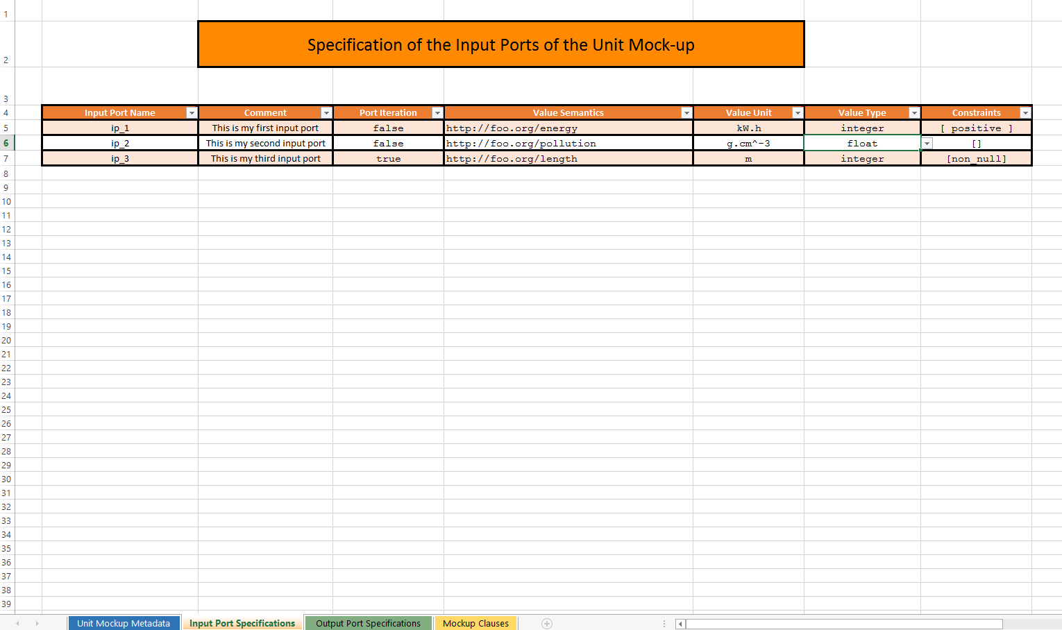
Third, the definition of its output ports:
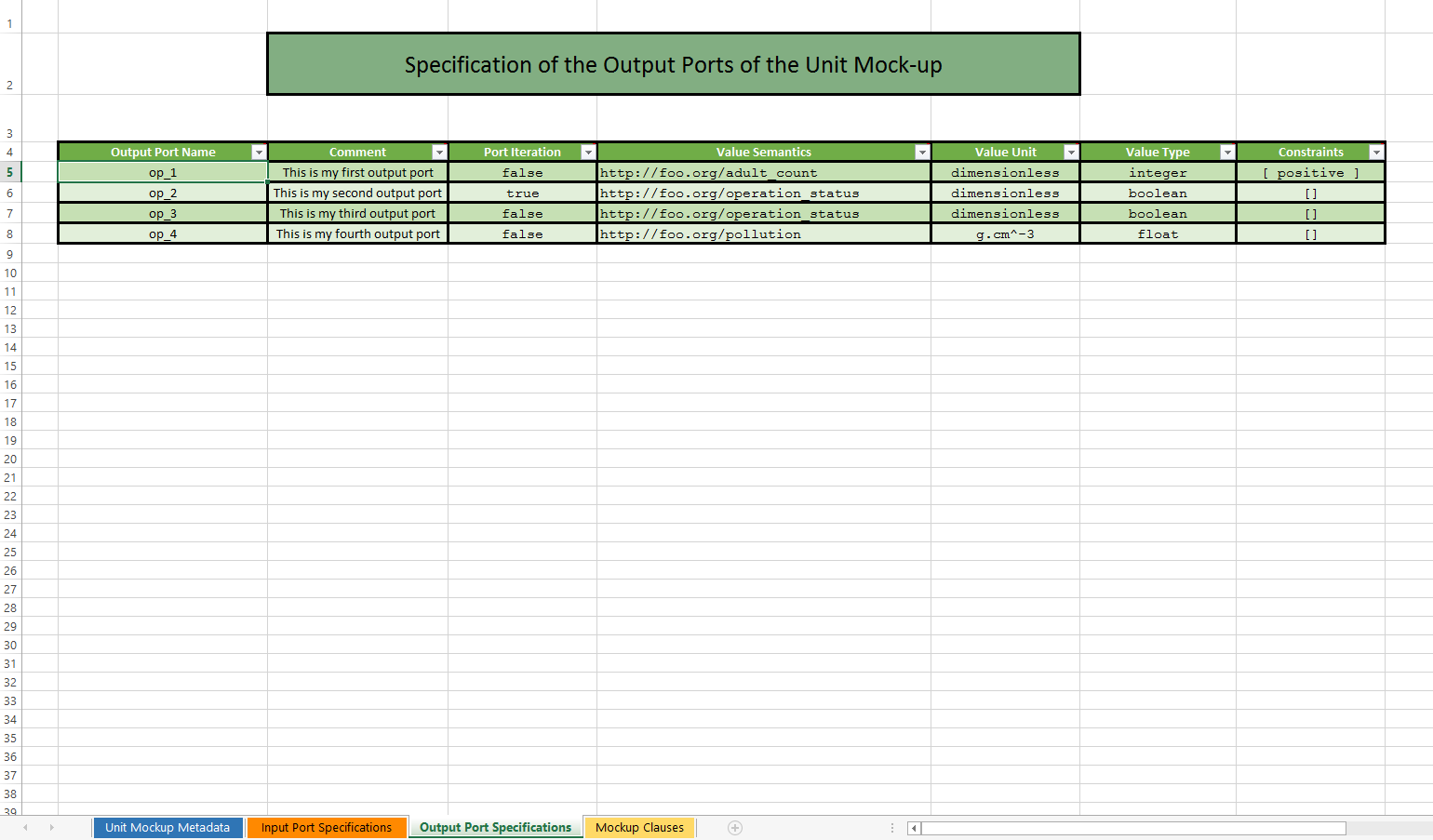
Finally, the definition of its mock-up clauses, specifying the outputs that shall correspond to specific times and inputs:
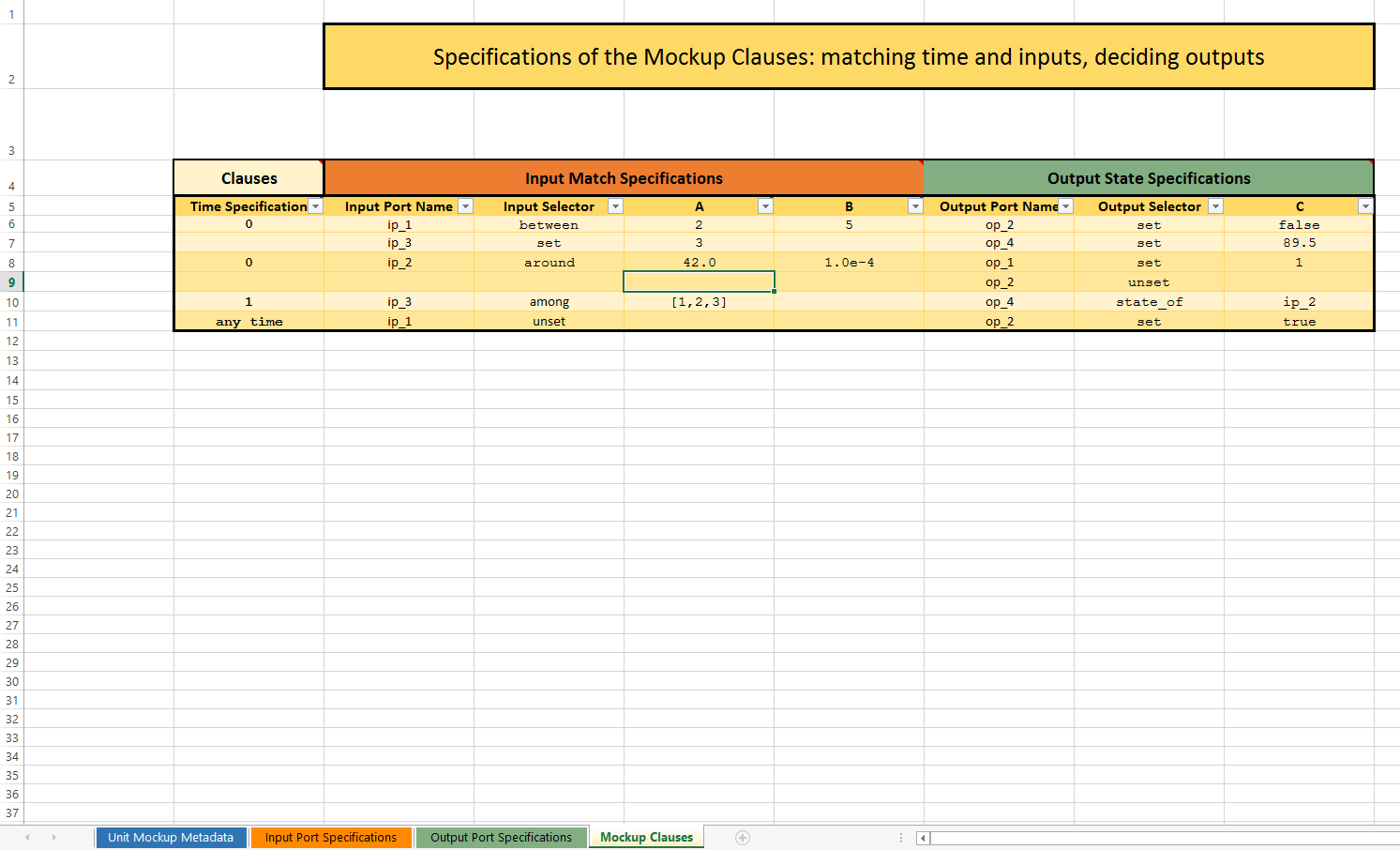
A few Supplementary Pieces of Advice
- inside the metadata worksheet, the first version listed (Version of the Dataflow Unit Mockup Format) is read-only, as it is the current version of the mock-up format (not the version of the particular mock-up being defined; for that see the Version of the mock-up metadata instead); please ensure you are always using a spreadsheet template in the latest, stable version of this DUMF format (otherwise it is bound to be rejected by tools that are in more recent versions)
- the overall structure of the Excel spreadsheet and each of worksheets are protected (locked by default), to avoid erroneous user-originating changes; they can nevertheless be unlocked thanks to the dataflow password; use it with care!
- semantics shall be always specified; a warning is emitted otherwise
- exotic, Unicode characters shall be avoided; otherwise a warning will be issued and the corresponding string will be replaced with (non-ASCII string)
- when defining a boolean value, it should be specified as following strings: either "true" or "false" (we recommend not to use Excel-defined boolean constants, which are represented as TRUE / FALSE, VRAI / FAUX, etc.)
Possible Enhancements
- the patterns recognized could include the state of another input port (e.g. {I4,I6} meaning that I4 should be in the same state as I6), of course provided that the dependency graph remains acyclic
- port names could also be pattern-matched; for example an input match spec could include {"ip_*",{set,3}} to specify that any input port whose name is prefixed with ip_ and that is set to 3 would validate this part of the match
- during a time-step, a given unit might be triggered any number of times (from none to more than once); even if introducing logical moments (i.e. replacing timesteps with a pair made of a timestep and a logical moment, i.e. a diasca) is probably not desirable, maybe specifying whether a unit is allowed to be triggered once (once) or any number of times (always) could be useful
Integrating a Model As a Dataflow: a Short Walkthrough
So you've got a Foobar model, maybe pre-existing, maybe just specified, and you want to integrate it in a more general dataflow? Here is a list of simple steps to go through in order to ease that integration.
For the sake of example, let's suppose that this Foobar model performs energy-related assessments in the context of cities.
Preliminary Step (#0): Remembering the Basics
Let's recap first the general structure that we target and the features we need to support.
A model embodies computations of some sorts (for example, here, some energy evaluations) that are intermingled with others (e.g. there may be interrelated evaluations about waste or transportation), the whole applying to the state of a system (e.g. a city) and updating it in turn (e.g. all these evaluations are performed for a given year, and the dynamics they capture will lead to an updated city, available for the next simulated year).
To turn such a simulation into a dataflow, both the state of the system and the computations performed on it have to be modelled thanks to dataflow constructs.
Here the state is typically modelled based on Dataflow Objects (e.g. the city as a whole may be hierarchically divided into districts, buildings, households, etc. - each of these urban objects being represented by a dedicated dataflow object instance).
The main role of these dataflow objects is to store, thanks to attributes, the relevant state information of these various parts of the system so that the expected computations can be carried, i.e. so that these computations can be fed with the data they need and so that they can as well update that state with their results. As a consequence, prior to the integration of the computations, an agreement on the structure (based on dataflow objects) and on the content (based on the attributes of these objects) of the description of the system at hand shall be found.
As for the computations (including the ones provided by the Foobar model), they are to be described macroscopically in terms of a set of Dataflow Processing Units (e.g. a type of unit can correspond to the energy evaluation, whereas another type of unit may take care of waste and transportation).
Of course multiple instances of a given type of unit may exist to account for the underlying multiplicities of dataflow objects. For example, if some computations have to be done strictly on a per building basis, then a corresponding processing unit type may be defined, and a bijection (a one-to-one relationship) between buildings and such unit instances should exist.
Moreover one can note that not only a given unit type may be instantiated more than once, but also that such a unit may have to be created and deleted dynamically, in the course of the simulation. In our example, on a given simulated year the creation of a building in the city shall result in the creation of a related instance of our unit type; conversely, destroying a building shall imply the deletion of its associated unit instance.
Finally, whether or not urban objects are created or deleted, connections between dataflow elements (processing units and urban objects) are in the general case bound to be modified over simulation time.
These unit-level operations (creation, connection, update, deletion, etc.), whether they are done initially or in the course of the simulation, are to be driven by dedicated unit managers - whose design and implementation must be planned as well.
Step #1: Ensure that the Overall Simulated World Can be Structured As a Dataflow
In this step we want to retain a clean dataflow approach in order to:
- describe the Foobar model as a whole
- insert in its context
At this step we still see the Foobar model simply as a single, monolithic logical unit. We specify here only what are the "high-level" computation features that each of the units involved in the dataflow offers and the information that each unit requires (not how precisely units are to operate internally).
The purpose of this step is:
- to cleanly separate the single, consensual description of the system state from the usually multiple, diverse computations that shall be operated on it; the crucial point is that this state must be defined so that it provides all the information needed by all computations to be operated (those of Foobar and the ones of all other units) - and preferably only them, while keeping these pieces of data orthogonal, i.e. avoiding any duplication of information [38]
- to establish how these computations are organised - including the ones that are to be taken in charge by this Foobar model
- to express the whole uniformly, and in terms of dataflow constructs (objects and processing units, and also streams of information)
| [38] | For example any needed living space attribute of a (dataflow object) building shall be defined once for all, instead of introducing as many (attribute) variations of it as there will be different unit types requiring such an information. Otherwise the state of dataflow objects would be bound to become increasingly difficult to maintain, if not silently inconsistent (e.g. one version of the livable surface being updated while the others not). |
Step #2: Determine the Specific Relationships Between the Dataflow and this Model
At this step we concentrate on the Foobar model and on the units in direct relationship with it.
There will be indeed actual connections between this black box of interest and the rest of the dataflow: the Foobar model is to be fed by inbound dataflow channels, and reciprocally outbound channels are to stem from this box and feed other elements of the overall dataflow.
This step requires that all dataflow elements in direct interaction with the Foobar model box (whether they are upstream or downstream) are listed and specified in terms of connectivity with Foobar: the corresponding channels shall be named and defined, with their multiplicity and their corresponding SUTC information.
The list of input and output ports that should be ultimately provided by the logical unit corresponding to Foobar are to be then determined from these channels.
An added bonus of completing this step is that it enables the possibility of defining a mock-up for that Foobar model: now that it is more formally specified as a self-standing component, one is able to devise input and output datasets that can emulate its behaviour as a whole. See the section about mock-up units for more details.
Alternatively, the completion of the next step might be awaited, so that individual units corresponding to this model can be each represented by a dedicated mock-up.
Step #3: Break the Black Box Into Actual Dataflow Units
In the previous steps, the Foobar model was seen as a single black box (one "abstract", logical unit). Now is the time to break the Foobar black box into pieces, and to express them as a set of actual dataflow blocks.
Indeed, in the general case, for each model multiple dataflow units are needed in order to account for the various computational stages and multiplicities that a model must support.
For example, some aggregations (e.g. spatial ones) are often to be done before and after the central, domain-specific computations of the model, and for that they need a varying (runtime-determined) number of input and output ports (e.g. an instance of the Foobar model may have to accommodate for any number of energy sources).
If simple models may be expressed only thanks to a single processing unit relying on port iterations, more complex models often require to be translated into a set of interlinked dataflow units, some of which taking in charge the bulk of the computations while others are in charge of transforming (e.g. aggregating, summing, averaging, converting, routing, etc.) information on their behalf.
So the outcome of this step is to have a design of the Foobar model once it has been translated into a collection of actual dataflow units whose superposition provides the combined input and output ports that have been determined in the previous step.
Step #4: Implement the Corresponding Actual Units
Now that the Foobar model has been split into real, dataflow units, in the general case these units do not exist yet, and thus have to be implemented [39].
| [39] | Depending on the history of the project, some already available units may be re-used. Similarly, some units may perform fairly standard operations (e.g. simple aggregations) and thus may be provided by the dataflow infrastructure as built-in. Usually at least the model-specific computations must be developed. |
Each newly-introduced processing unit can either be a native unit (i.e. written in Erlang and thus directly developed within the dataflow infrastructure), or a unit relying on a language-specific binding.
In this latter case, depending on the programming language that has been preferred, the unit developer will typically rely either on the Python dataflow binding or on the Java one. In both case the provided dataflow API must be used in order to define the new unit.
In practice, it boils down simply to:
- making this new processing unit inherit from the base dataflow unit type
- defining the construction parameters needed to create a new instance of such a unit
- specifying accordingly what its input and output ports are (number, name, whether they are iterations, SUTC information, etc.)
- defining how this unit should be activated (typically whether the setting of any, or all, of its input ports is needed)
- defining what the unit should do when it is activated (typically read at least some of its input ports that have been set, compute elements from them and from its state, possibly update in turn some of its output ports and its own state)
Step #5: Add the Corresponding Unit Manager(s)
The previous steps led to the availability of the whole implementation for the Foobar model: now, for this model as well, the overall dataflow objects bear all necessary information (step #1), its connectivity has been established (step #2) and its complete counterpart in terms of dataflow units has been designed and implemented (respectively step #3 and #4). Therefore we defined how the Foobar model is to be evaluated once properly set-up.
This last step (#5) consists on the definition or update of the associated unit manager, in charge of the correct insertion and management of the units corresponding to Foobar in the overall dataflow.
This includes at least how its units shall be created and linked whenever an instance of the Foobar model is needed; various dataflow-level events may have to be supported by a unit manager.
In our example, the Foobar unit manager should be able to be notified that a new building (dataflow object) has been created, so that this manager can create in turn the appropriate new instance of Foobar: the unit manager should ensure that the various units for Foobar are then correctly instantiated and also connected (between themselves and also with the rest of the dataflow).
Requirements For the Dataflow Integration of a Model
- R1: a description of the overall dataflow must be defined, in which the target model is represented by a single, abstract, dataflow unit; its inbound and outbound channels shall be specified
- R2: the target model itself shall be defined in terms of dataflow constructs
- R3: the general operational rules apply (e.g. compliance with the underlying operating system and libraries)
Implementation Section
Mode of Operation
As already mentioned and represented in the class diagram below, processing units are implemented as instances of the DataflowProcessingUnit class, a child class of the DataflowBlock one, itself a child class of the basic (Sim-Diasca) Actor one (note that, actually, all classes represented on this diagram are child classes - directly or not - of the Actor one).
Most units are passive actors: they will be solely scheduled if/when some of their input ports are triggered, which, depending on their policy, might result in their activation. Some units (e.g. source ones) may be active, in the sense that they may choose to develop a spontaneous behaviour (typically to auto-activate periodically).
A special case of unit has been defined, the DataflowMockupUnit. Such mock-up unit provides a generic emulation of a unit, associating output values to input ones based on the data (rules) it has been provided with. It is typically used to develop termination plugs that allow to wait until the implementation of the final unit is ready, and to validate it afterwards.
Ports (input and output ones alike) are mere data-structures (records) held by their block (maintaining an associative table for both of them).
We propose the following convention to name the variables holding a port:
- the name of the variable shall reflect the name of the corresponding port (e.g. if the port is named "My distance", the variable name may begin with MyDistance
- if it is an input port, the variable name may end with IPort (e.g. MyDistanceIPort)
- if it is an output port, the variable name may end with OPort (e.g. MyDistanceOPort)
Implementation-wise, channels do not exist per se, they are abstracted out thanks to ports.
The static channel-related information (e.g. SUTC, for semantics, unit, type, constraints) is held by all endpoints (the output port and its linked input ports); as their metadata are checked for compliance when ports get connected, the exchanged values do not include them, since they are automatically checked in turn for compliance at port sending and receiving.
Dataflow values are records that store their accuracy, timestamp and, of course, actual value. As always, they are exchanged through actor messages, managed by the engine.
As for the dataflow objects, they unsurprisingly inherit from the DataflowObject class. These actors participate to the description of the simulated world and, thanks to their dataflow attributes (special actor attributes that map to a pair of input and output ports), they are ready to be integrated in a dataflow.
Finally, instances of dataflow objects of a given class (e.g. Building) are governed by a dataflow object manager specific to this class (e.g. BuildingManager). All these managers inherit from the DataflowObjectManager base, abstract class.
Similarly, all instances of a given type of unit (e.g. EnergyDemand) are governed by a unit manager specific to this class (e.g. EnergyDemandManager), and all these managers inherit from the UnitManager base, abstract class.
The overall dataflow could have remained implicit (in the sense that no specific instance could have been defined in order to designate it as such, a dataflow being just an abstract concept corresponding to a set of actual, interconnected blocks), yet having it in an explicit form (i.e. as an instance of a well-defined Dataflow class) has been deemed more convenient and future-proof.
So we end up with the following dataflow-related class hierarchy:
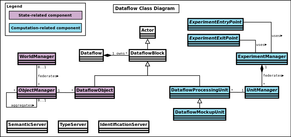
Usage: Defining One's Dataflow
Preferably an overall schema of the dataflow is determined first. One must keep in mind that a dataflow is a graph of computations, i.e. a description of interlinked tasks, processed by units, possibly fueled with information from objects.
Then, for each type of unit (as of course a dataflow may include multiple instances of the same unit), a child class of DataflowProcessingUnit shall be defined.
The actual processing done by that kind of unit is to be implemented by overriding its activate/1 method. It will be based on the unit state, including the value carried by its input ports that are set. In some very rare cases, a spontaneous behaviour might be defined as well, if appropriate for that unit.
Any dataflow object used shall also be defined, which mainly consist on defining its (dataflow) attributes.
Once all object and unit classes are available, the target dataflow instance can be built. This is done by creating first the relevant block instances (either from a data stream listing their construction parameters, or programmatically), interconnecting their ports and registering themselves to their federating dataflow.
Then, once the simulation is started, some source blocks are expected to get activated (possibly thanks to active blocks, or to explicit block activation); their triggered ports shall in turn activate other blocks and trigger other ports, animating the whole dataflow so that it performs the processing that is expected from it.
Please refer to the Dataflow Urban Example, whose sources are located in the mock-simulators/dataflow-urban-example directory, for a full source of inspiration.
Class or Instance-level Checking
Any given instance dataflow block (e.g. a processing unit) may declare ports, statically or not.
Ports created statically are usually the same for all instances of that type of dataflow element. So, instead of performing checks (e.g. in terms of semantics or types) for each of these instances (that are potentially very numerous), the verification is better done once, at the class level - based on its declarations.
For example, for units, any of them should preferably declare statically these information so that its unit manager can check them at simulation startup [40].
| [40] | See class_DataflowElementActor:declare_static_information_for/1. |
To establish whence semantics and typing information come for a given dataflow element, the following rules apply:
- for semantics:
- any kind of semantics can be reported by this type of dataflow element by having it define and export its get_declared_semantics/0 static method [41]; this may be a way of specifying the semantics both for the initial ports and for any other port that may be created in the course of the simulation (if specified, must be exhaustive)
- otherwise (if no get_declared_semantics/0 method is exported), the semantics may be deduced from its get_port_specifications/0 static method, if of course it has been defined and exported
- otherwise, the element does not report any semantics
- for types, a slightly different logic applies: the get_declared_types/0 static method should be used whenever having to introduce new types, especially so that the types mentioned through get_port_specifications/0 can be resolved
| [41] | For semantics, their name is also their definition (e.g. 'my semantics'), whereas types have to be specifically defined (e.g. my_type is [integer]) before being used (e.g. my_value is of type my_type). |
Defining get_port_specifications/0 is recommended, as by design the static information that is reported matches the ports that are initially created. Otherwise explicit checking shall be done when creating the actual initial ports, to ensure their information match any one that would be statically defined thanks to get_declared_{semantic,type}s/0.
Finally, some amount of runtime checking may still be necessary, as ports may be created dynamically.
Scheduling Cycle of Experiments
The logical order of the operations involved in the step-by-step evaluation of an experiment has been presented in the section about Experiment Progress.
However dataflows may be arbitrarily complex computation graphs, with various branches and, potentially, cycles, so detecting when the intra-tick evaluation of a given dataflow is over (i.e. when none of its blocks can be triggered anymore) is not straightforward, as this consists mostly in detecting the absence of an event.
The solution elected here, in technical terms, consists on inducing an offset in this three-stage cycle (experiment entry/dataflow evaluations/experiment exit).
Indeed, at each new tick, the experiment exit point is triggered first (obviously not doing anything for the very first tick); it is the only actor here having a spontaneous behaviour.
It then triggers (as always thanks to an actor message) the experiment entry point, which performs the tick-specific initialisations. This usually leads to the update of various dataflow elements and thus to the evaluation of various dataflow for that tick.
Once none of the dataflow elements set any output port, no other dataflow element can be triggered anymore (no more diasca created), hence the engine determines that this tick is now over, and schedules the next planned one.
Then again the experiment exit point is scheduled and is free to perform any termination action for the dataflow evaluations made at the previous tick. Then it triggers the experiment entry point, which triggers the dataflow evaluations again, and so on.
Life Cycle
The goal is to rely on a single, shared evaluation infrastructure (taking in charge by a relevant set of singleton managers) allowing for multiple dataflow instances (each with its own object and unit instances).
As a consequence, the dataflow blocks (i.e. the actual dataflow objects and units) are:
- referenced by their top-level respective managers (i.e. the world manager and experiment manager, which maintain a per-class list of instances)
- owned by the dataflow to which they are registered (which may then delete them appropriately)
As for the various object and unit managers, they are owned by, respectively, the world manager and the experiment one.
Note that all the classes involved here:
- class_Dataflow
- class_Dataflow{Block,Object,ProcessingUnit}
- class_Dataflow{Object,Unit}Manager
- class_Experiment{Entry,Exit}Point
- class_{Experiment,World}Manager
are child classes of the class_Actor one, and as such will have their instances automatically removed at simulation end.
Implementation Details
The dataflow constructs are defined, in the code base, in the sim-diasca/src/core/src/dataflow source tree.
Traces sent by the dataflow architecture are available in the Core.Dataflow category and its children categories.
A dataflow initialization file has preferably for extension .init (e.g. dataflow-urban-example.init).
It generally lists the creations of:
- the relevant base components, i.e. the WM and its dataflow object managers, the EM and its dataflow unit managers
- at least one dataflow
- the relevant actual instances of dataflow objects and processing units
Appendices
Annex 1: Design Questions
- Should all output ports of all blocks of the dataflow emit at each diasca a value, even if it did not change (event-based or synchronous)?; if yes, many useless sendings and schedulings, and not all units have the same temporality, so a year-based one, if included in a simulation with a daily one, would have to change its behaviour; so we preferred opting for an event-based mode of operation
- As not all state changes/operations are instantaneous, should delays (in diascas or ticks) induced by a block be managed? (e.g. ignition spark received, explosion happening 4 milliseconds afterwards)
- Would it be possible and useful that units can be composed, i.e. that a given unit can actually be recursively made of sub-units? If such a feature was wanted, then ecore could be used to define the corresponding system, and two different approaches could be considered:
- either defining, directly at this dataflow level, nested units, and manage the consequences thereof (e.g. when the inputs of a "macro" unit would change, its outputs would change in turn accordingly, yet only after some delay in terms of logical moments (i.e. only once some of them elapsed, with state transitions that may be arbitrarily deferred)
- or introduce new, higher-level concepts, such as the one of assemblies that can be nested; an assembly would ultimately translate to a basic, non-nested dataflow, by collapsing a (multi-level, compounded, compact) assembly into a (single-layer, uniform, intricate) dataflow; for that assemblies (either user-defined or generated) would be recursively unboxed and expanded into their parts until only standard dataflow blocks are found (a bit like when going from a higher-level electronic schematics to its full, elementary counterpart at the level of the logic gates)
- Should large datastructures have to be carried by channels, maybe these data currently pushed by an output port shall be pulled by the input ports instead? (anyway this will most probably lead to a term duplication anyway)
- If a model deals with a currency (e.g. euros, or US dollars of year 2012), is the best approach to have its unit flagged as dimensionless (hence, not euro) and complement this information at the semantics level?
Annex 2: Possible Overall Improvements
- knowing that a given type of unit, thanks to its constructor, can be parametrised (leading to its instances behaving differently), this may be represented graphically: instead of designating a unit type as FoobarUnit, it may be shown as FoobarUnit(height,width,color)
- a type of bus may be named (defining an ordered list of channel types); afterwards, one may consider bus auto-grouping, i.e. having a transparent translation of a bus-as-a-graphical-symbol (thus with N channels underneath) into a single pseudo-channel conveying a N-element tuple containing the related channel values (thus relying on one sending instead of N)
- a group of ports (portset?) may be represented by a unique, conventional graphical element (a portset is to ports what buses are to channels); more specific activation policies could rely on portsets
- scale hints could be revamped (as a unit may have one scale, its inputs others, and the same for its outputs)
- a consensual, sufficiently expressive language of types should be defined and enforced all the way regarding the values conveyed by the dataflow (such a check is not done currently)
- the state changes of a dataflow may be collected by a process (should this feature be enabled), which could either write them in a file according to a conventional format (e.g. *.df-state) or make them available through an ad-hoc http server; in both cases, these information could feed a tool representing graphically (according to the conventions listed in annex 3) the state of a dataflow (as an image), or the changes over time of the state of a dataflow (as a video made out of frames, generated with as few layout changes as possible from one to the next)
- a support for a Python implementation of unit managers (at least the simplest/most classical ones) could be provided
Annex 3: Conventions for the Graphical Representation of Dataflows
Example Diagrams
When having to represent a given dataflow of interest (typically in a design phase), to favour consistency we recommend that one starts from the diagrams we already made for this document and for the base examples.
For that, one shall use Dia, a free software diagram editor.
Our dataflow-diagram-toolbox.zip [42] archive centralizes the best examples for such a reuse, from which more homogeneous user diagrams can be easily derived.
| [42] | This archive can be generated from sim-diasca/doc/dataflow-howto by running make. |
Later, a specific Dia library for dataflows could be devised (should no higher-level tool be available then).
Color Charter
Here are the color definitions that we recommend to respect, for clarity (when two colors are specified, the first is a lighter version of the second):
| Elements to Represent Graphically | Associated Color | Color RGB Definition |
|---|---|---|
| Input ports | Dark orange | ffcd70 / ff8900 |
| Output ports | Dark green | 688e68 / 82ae82 |
| Channels, buses and port-level meta-data | Pure blue | 0000ff |
| Lines for shapes (e.g. units) | Pure black | 000000 |
| Default background | Pure white | ffffff |
| State-related background | Light purple | f1e3f1 |
| Dataflow object | Stronger purple | cfaecf / a13ba1 |
| Computation-related background | Light blue | e1ebff |
| Dataflow unit | Stronger blue | 96d2e6 / 0000ff |
| Scale indication background | Light yellow | faf8b3 |
| Probe | Blue | 3838f4 |
| Post-it like comment | Lighter yellow | ffffc8 |
Buses (i.e. sets of channels) are represented like channels, yet thicker (generally, their line width is to be equal to 0.10 cm times the number of channels they regroup) and barred with a dash (a bit like in electronics), with the channel count being displayed just above.
Both channels and buses may adopt different colors (preferably blueish, though) to help the reader understanding the overall connectivity.
Annex 4: Credits
Many thanks, among others, go to:
- Samuel Thiriot, for many inspiring comments and ideas
- Omar Benhamid, for rich exchanges about the entry and exit points of a dataflow
- Robin Huart, notably for the mock-up units, the language bindings and the platform integration
- Karel Redon, for thoughts about the buses and their graphical representation, and for the Python workbench