Technical Manual of the Sim-Diasca Simulation Engine

Organisation:Copyright (C) 2008-2024 EDF R&D
Author:Olivier Boudeville
Contact:olivier (dot) boudeville (at) edf (dot) fr
Creation date:Monday, February 8, 2010
Lastly updated:Tuesday, February 13, 2024
Version:2.4.7
Status:Stable
Website:http://sim-diasca.com
Dedication:For people interested in the inner workings of the Sim-Diasca simulation engine.
Abstract:The main design choices of the simulation engine are discussed here, from the requirements to the implementation, including the software architecture and the algorithmic approach. Its recommended use is also described.

Table of Contents

Note

Before reading this document, we strongly advise to have a look first at the slides of the general-purpose presentation of Sim-Diasca.

Overview & Context

Sim-Diasca

Sim-Diasca stands for Simulation of Discrete Systems of All Scales.

Sim-Diasca is a lightweight simulation platform, released by EDF R&D under the GNU LGPL licence, offering a set of simulation elements, including notably a simulation engine, to be applied to the simulation of discrete event-based systems made of potentially very numerous interacting parts.

This class of simulation encompasses a wide range of target systems, from ecosystems to information systems, i.e. it could be used for most applications in the so-called Complex systems scientific field.

Before entering in the details of the present manual, we recommend the reader to go first through the Sim-Diasca general-purpose presentation in order to benefit from a general overview.

As a matter of fact, a classical use case for Sim-Diasca is the simulation of industrial distributed systems federating a large number of networked devices.

The simulation elements provided by Sim-Diasca are mainly base models and technical components.

Models are designed to reproduce key behavioural traits of various elements of the system, notably business-specific objects, regarding a specific concern, i.e. a matter on which the simulator must provide an answer. An instance of a model is called here an actor. A simulation involves actors to be driven by a specific scenario implemented thanks to a simulation case.

Sim-Diasca includes built-in base models that can be further specialized to implement the actual business objects that are to be simulated.

Technical components allow the simulator to operate on models, so that their state and behaviour can be evaluated appropriately, in the context of the execution of an actual simulation.

Depending on the conventions that models and technical components respect, different properties of the simulation can be expected.

Thus the first question addressed in the context of Sim-Diasca has been the specification of the simulation needs that should be covered, i.e. its functional requirements.

Then, from these requirements, a relevant set of technical measures has been determined and then implemented.

Current Status

Sim-Diasca and the first simulators making use of it are works in progress since the beginning of 2008, and the efforts dedicated to them remained light yet steady.

The Sim-Diasca engine is already fully functional [1] on GNU/Linux platforms, and provides all the needed basic underlying simulation mechanisms to model and run full simulations on various hardware solutions.

A set of models, specifically tied to the first two business projects making use of Sim-Diasca, have been developed successfully on top of it, and the corresponding business results were delivered appropriately to stakeholders.

[1]This is also a great pun, as the simulator is implemented thanks to the Erlang language which, in terms of programming paradigm, is a functional language.

Some further enhancements to the Sim-Diasca engine are to be implemented (see Sim-Diasca Future Enhancements).

Minimal Quick-Start For Early Technical Testing

For the fearless users wanting an early glance at Sim-Diasca in action, here is the shortest path to testing, provided you already have the prerequisites (including a well-compiled, recent, Erlang interpreter on a GNU/Linux box) installed.

First, download the latest stable archive, for example: Sim-Diasca-x.y.z.tar.bz2.

Extract it: tar xvjf Sim-Diasca-x.y.z.tar.bz2.

Build it: cd Sim-Diasca-x.y.z && make all.

Select your test case: cd sim-diasca/src/core/src/scheduling/tests/, for example: scheduling_multiple_coupled_erratic_actors_test.erl.

Optionally, if you want to run a distributed simulation, create in the current directory a file named sim-diasca-host-candidates.txt which lists the computing hosts you want to take part to the simulation, with one entry by line, like (do not forget the final dot on each line):

{'hurricane.foobar.org', "Computer of John (this is free text)."}.

Then run the test case:

make scheduling_multiple_coupled_erratic_actors_run CMD_LINE_OPT="--batch"

The CMD_LINE_OPT="--batch" option was added as, for the sake of this quick-start, the trace supervisor is not expected to have already been installed.

For the more in-depth reference installation instructions, refer to the Sim-Diasca Installation Guide.

How to Read This Manual

Let's Start With A Short Ontology

What is an Ontology?

As defined here, an ontology formally represents knowledge as a set of concepts within a domain, and the relationships among those concepts. It can be used to reason about the entities within that domain and may be used to describe the domain.

We aim here to express a Sim-Diasca ontology about (discrete-time) simulations of complex systems, so that we can define relevant terms and share them once for all.

Simulation Concepts in Relation

Many additional relations could be defined, we just concentrated on the most influencial ones. Each concept is defined in turn at the bottom of this diagram.

Simulation Terms Defined

The ontology is currently in a simpler form, the one of a glossary (terms, sorted alphabetically, and their definition).

The examples illustrating the definitions are taken from a hypothetical simulation case involving preys and predators (a typical use-case in this simulation domain).

Abstraction
An Abstraction is a simplification of elements of the Simulated World regarding traits of interest, i.e. how the Simulation should represent a part of the various elements to be simulated. An Abstraction is a Schedulable. Typically an Abstraction is either a Modlet or a Scenario.
Actor
An Actor is an instance of a Modlet. For example: "This particular actor corresponds to this specific prey that we wanted to introduce in previous simulations, the one that is bound to be eaten first due to its starting location."
Experiment settings
An Experiment settings is a set of runtime static parameters that applies to all instances of a given Abstraction in the context of a given experiment (i.e. Simulation). Indeed, when constructed, Abstractions may accept a set of parameters that will be common to all their instances for that simulation. It is a way of overriding, at the level of a given simulation, the internal constants ruling the Abstraction behaviours. A key point is that these parameters are static, i.e. that, on a given simulation, they apply to all instances of a given Abstraction, while another simulation may rely on other experiment settings (the default ones or other overriding parameters). Experiment settings are known in some simulations as "strategies". For example an Experiment settings may define various constants that determine the efficiency of the technical elements making up a kind of photovoltaic panel. All instances of the corresponding Modlet will share these Experiment settings, but these settings may differ from one simulation to another (e.g. a given technology could be made more cost-effective in another simulation relying on a different context).
Model
Model designates primarily an overall system (often the Target system as a whole), like a city - even if in the simulation there is no specific instance corresponding directly to that name (e.g. not even a City Modlet defined; for example a city could be then represented in such a simulation just as a set of building instances instead). By extension a Model may also be used as a synonym of Modlet (see next entry), an actual simplification of an element of the Target system. It is a type (like a class), from which instances (Actors) can be created; it then defines notably their state and behaviour. For example, "I am quite happy of the current predator model, it behaves nicely compared to what experience tells us. See how its instances are chasing these preys?" As the target system, which is reproduced thanks to a collection of modlet instances (second acception of Model), can be itself seen as a Model (as defined in the first acception), the term may be ambiguous in some contexts. In these cases, Modlet should be used only to designate the type of actors (the implemented, disaggregated parts of this overall model), while Model would be used for more conceptual descriptions (that are not instantiated as such). When there is really little ambiguity, Model may be used to refer to Modlet, but it is not encouraged.
Modlet
A Modlet is an atomic sub-model of a simulation, i.e. a modeling element that cannot be further simplified and corresponds directly to a type that can be instantiated. In following example there is no specific city instance as such: “This tiny model of San-Francisco involves only a few building modlets, some road modlets and three bridge modlets.” A set of Modlets may form a more general Model, possibly the overall one.
Probe
A Probe is a producer of simulation results, based on information made available by a set of Abstractions. For example, "I need to monitor how many preys are killed by predators of this type. I will add a probe to track this information". A probe may be fed by multiple abstractions.
Scenario
A Scenario is a representation of the elements in the Simulated world that are outside of the Target system but that may influence it and/or possibly be influenced by it. For example, "My monsoon scenario, once combined to your epizootic scenario, shows unexpected results in terms of prey population." The set of all Scenario instances form the System context.
Scenario instance
A Scenario instance is simply an instance of a Scenario, like an Actor is an instance of Modlet. Scenario instances and Actors are technically managed the same way; their difference lies in the viewpoint of the author of the simulation, who can arbitarily set the limit between the system of interest (the Target system) and its surroundings (System context).
Schedulable
A Schedulable designates any element that is driven, time-wise, by a Time manager, like Abstractions.
Simulated world
The Simulated world corresponds to the full set of Abstractions that are to be evaluated through the simulation; the Simulated world is the union of the Target system and its context (i.e. the System context), i.e., respectively, Actors and Scenario instances. For example, "The simulated world is the whole savannah, including fauna and flora."
Simulation
A Simulation corresponds to the execution of a Simulation case. It is an experiment typically done for decision-making.
Simulation case
A Simulation case is the specification of a Simulation. This encompasses: - Technical settings, like the properties to be enforced for this simulation (e.g. reproducibility), the time-step to be used or the list of the eligible computing hosts - Domain-specific settings, like the description of the initial state of the simulation or its various termination criteria For example, "This predator / prey simulation case, which must run on these following 3 computers, will rely on a 20 millisecond timestep; it takes place in this kind of savannah and starts with 2 predators (that can mate) and 15 preys, on these specified locations. This is the weather scenario that I want to apply. I want the simulation to stop whenever either all animals are extinct or the elapsed duration (in simulation time) reaches one century. In terms of results, I want the simulation to keep track only of the predator population and of the number of preys that are born in its course."
Simulation engine
The Simulation engine is, among other roles, in charge of managing the virtual time of a simulation; by scheduling the various Schedulable instances, it allows to enforce the properties expected from the simulation while making its (virtual) time progress, preferably in an efficient way. Typically a simulation engine includes a Time manager service, which is a key feature thereof.
Simulation inputs
The Simulation inputs correspond to the data that is needed for the simulation to be ready to start. This encompasses notably the description of its initial state, i.e. the data allowing defining the state of the whole simulated world when the simulation is to begin.
Simulation outputs
The Simulation outputs regroup the simulation results and the simulation traces (we consider here only successful simulations - failed ones output errors and traces).
Simulation results
The Simulation results are the main by-product of a simulation, if not its only purpose. These are data that are computed based on information provided by Actors and Scenario instances, at various points in Simulation time, and that are aggregated and managed by Probes.
Simulation time
There are at least two kinds of time that are useful in the context of a simulation: the wall-clock (user) time (i.e. the one we, humans, all experience) and the Simulation time that is known of the simulation, i.e. of actors and scenario instances (a.k.a. the virtual time the Simulated world is plunged into; at least a discretised version thereof). By default there is no link between the wall-clock time and the simulation one.
Simulation traces
The Simulation traces correspond to the time-stamped (in wall-clock or simulation time) information emitted by the actors, scenario instances and the technical agents of the simulation, during its course (e.g. probes, service providers). These are not simulation results, they are a technical means of following the events that happen in the course of a simulation, for example in order to troubleshoot the behaviour of models.
System context
The System context gathers everything in the Simulated world that is not the Target system. It is made of all the Scenario instances.
Target system
The Target system is the system of interest, whose mode of operation is reproduced thanks to a set of models. Generally such a target system cannot be simulated without its context, i.e. parts of the reality that do not belong to the target system but must be taken into account to simulate it. For example, "The target system is made of the preys and the predators. Its context is the weather and the savannah (vegetation and relief)."

Sim-Diasca Specifications

Sim-Diasca has been originally designed in the context of two French and British projects aiming to perform a massive roll-out of communicating meters for millions of residential customers.

This became a typical example of the complex systems whose simulation could be addressed by Sim-Diasca, showing the usual process involved by a project having to focus on business simulations: as the development of models and simulation cases is long and expensive, and as switching from an engine to another in the course of a project is almost never an option, an appropriate choice in the simulation tools is crucial for the success of such a project.

To reduce this technical risk, a very basic, straightforward decision process is generally to be applied:

  1. establish the functional requirements for the targeted simulator
  2. deduce and formalise the corresponding technical requirements
  3. make a review of the state of the art of this simulation field, and establish a short list of the most relevant simulation tools
  4. test and rank each of them against the list of needed properties that was previously agreed from step 2 and weighted accordingly
  5. elect the best candidate, possibly by benchmarking it on a representative use-case against a reference tool or the best other contenders

Simulator Potential Role

Note

In this document, we will often rely on examples taken from the smart metering field; however one must keep in mind that Sim-Diasca is a fully generic, business-free simulation engine, which has no connection at all with metering, and which can be applied to any kind of discrete complex systems.

In our context, the goal was to be able to perform virtual experiments on a system - here, before it even exists - mainly for decision-making purposes.

Indeed, the main purpose for such a simulator is generally to allow for a harmless test of a system:

[2]

[2]For the non-native English speakers, expressions like "SOH CAH TOA" are mnemonics for basic trigonometry.

(see the credits section about the comic strips)

Such a simulator could allow indeed to:

  • determine a priori some of the properties of the target system:
    • functionally, for example: "How are implemented the business services, with what overall coverage and constraints on the processes?"
    • technically, for example: "What is the lowest/mean/highest possible duration for this particular request to be completed?" or "What is the minimal bandwidth to plan for this particular link?"
  • compare answers to a call for tenders, so that the various solution candidates can be better evaluated
  • better review delivered versions of the system and ease their technical validation
  • help developing and tuning the system, for example by the impact on traffic due to a change in a data format
  • help validating project strategies, for example regarding the roll-out: "If meters are installed without any particular order, what is the ratio of meters whose proper operation could be directly validated at installation-time?"
  • quantify the costs of the system to establish its value analysis, by evaluating the total investments costs (e.g. for an installed concentrator) and operational costs (e.g. for GPRS communication costs, which may be partly proportional to the actual exchanged volumes)
  • better secure the ability of the system to evolve, for example by evaluating a priori the impact of a change in the functional or technical perimeter: "Should this new service be offered, what would be its technical feasibility (e.g. in terms of embedded processing or telecom link) and what would be the consequences on the overall properties and performance of the system?"
  • ease the test of all or part of the system, for example by recreating the environment of an actual component thanks to the simulation, and by assessing the correctness of the behaviour of the component with regard to a set of test interactions, which comply or not to the specifications

Of course any given simulator will rarely be requested to fulfil everything in such a wide range of expectations, but these are examples of questions that could be tackled thanks to a generic enough simulator and a set of appropriate models and metrics.

Simulator Potential Context of Use

Beyond the operational context of the aforementioned projects, such a simulator could be applied to:

  • R&D studies of alternative architectures for a metering system, for example:
    • offering different services
    • and/or based on other choices in terms of software architecture (e.g. showing a different dispatching of the processing on the various devices)
    • and/or using different infrastructures (e.g. mesh networks)
  • other target systems, like the one developed by the EDF supplier, instead of the one developed by ERDF, the monopolistic distributor
  • the British case, as a tool to help decision-making (EDF Energy, CLEVER project)
  • more generally, all kinds of simulation of information systems
  • more generally, all kinds of simulation of complex discrete systems

Functional & Technical Requirements

Here the simulation objective is to be able to rely on a simplified version of the target system, i.e. a model of it, on which various experiments can be conducted so that the overall system can be better understood, and questions about it can be answered.

We will discuss here the main requirements that applied to our use-cases and thus played a main role in the design choices for Sim-Diasca.

A Key Point: Scalability

Other Approaches Than Simulation Hardly Scale

Among the most challenging questions raised by this new system, many of them were directly related to the consequences of its significant size. And this same size prevented most of the usual evaluation approaches to be applicable. Indeed these approaches, which include:

  • thought experiments
  • expert-based assessments
  • simple extrapolations
  • more complex spreadsheet-based computations

could hardly tackle non-trivial questions since they generally fail to recreate precisely what happens in the system (notably time-wise) and what are the outcomes of these corresponding interactions: usually, only macroscopic values at equilibrium or not depending on time can be expected from these approaches.

Indeed some questions become increasingly difficult and crucial to tackle as the size of the target system rises: even simple individual behaviours, once interacting with a sufficient number of others, can combine themselves to form complex systems whose behaviour is surprisingly difficult to predict.

Solving issues affecting these systems is all the more difficult than some elements of a metering infrastructure, like the concentrators or the PLC networks, are themselves complex.

Despite these difficulties, such scale effects must be addressed soon, as costs induced by their late detection become quickly prohibitive.

Therefore the use of more demanding approaches like simulation is often needed, since, more often than not, a real-size target system cannot be built just for test purpose.

A Simulator May or May Not Scale

Due to the very large number of devices in most metering systems (more than 35 million meters in the French case), the simulator has itself to be able to scale up.

This does not necessarily imply that this tool must to be able to reach the exact full size of the target system, however it means it should be able at the very least to handle a massive numbers of interacting elements, as close as reasonably achievable to the real extent of the planned system.

Scalability is therefore at the heart of the properties wanted for that kind of simulators.

This concern severely constrained its implementation: so that it can reach performances suitable for its intended use, or just have a reasonable chance to actually deal with the problem in its required size, one had to ensure that the operation of the simulator is as concurrent as possible.

Concurrency First, But Other Properties Matter Too

The simulator had thus to be designed to be strongly parallel (on a given computation node, multiple models can be evaluated simultaneously by the available cores) and distributed (a simulation can take place over a set of networked computation nodes), and all this without hurting the properties deemed important but difficult to preserve in that context, such as:

  • the correctness of the evaluation of models
  • the preservation of causality between simulation events
  • the ability to have completely reproducible simulations

More precisely, in our case the objective was to rely on a framework, made of a generic simulation engine and of reusable components, that allows the development of simulations of information systems that are:

  • discrete rather than continuous, because the modeled phenomena themselves are essentially discrete, and those which were continuous could easily be quantized
  • in dynamic state rather than in steady state, since for example cascading outages or the progressive roll-out of the system are subjects of interest
  • event-driven, as state changes of the modeled instances are generally punctual and can happen at any time
  • causal, so that a total order on the simulation events can be recreated despite the massive concurrency
  • reproducible, so that different executions of the simulation take place identically, no matter their execution context, i.e. not depending on scheduling, dispatching of processing, available resources, number and nature of computing nodes, capacity of the network, etc.
  • intensely concurrent, as already mentioned, thus supporting a high degree of parallelism (taking advantage of multicores and SMP [3]) and able to be distributed over HPC [4] solutions like clusters or supercomputers (e.g. Bluegene)
  • potentially of very large scale, as already mentioned, to be able to simulate systems made of many thousands, if not millions, of interacting elements
[3]SMP: Symmetric multiprocessing.
[4]HPC: High Performance Computing.

This is the base specifications we had in mind for Sim-Diasca. However more generic and/or detailed requirements could be imagined, they are listed below.

List of Spotted Potential Properties For the Simulator

Determining the simulation properties that are required is a critical step of a project, so that an appropriate engine can be chosen. Indeed, the requirements may include very varying features to be provided by such a simulation engine, from high-level programming of models to scalability or support for continuous components (i.e. solver embedding).

The devil is in the details in terms of tool selection as well. So even two discrete simulation engines that, from a remote point of view, might look rather similar, may actually be widely different beasts.

Newly Added Properties

These properties and features were not listed in the initial requirements, but over time proved to be key points as well:

  • P21 Support for a complete result management, which allows mainly the user to specify what are the results expected from the simulation (preferably producing them, and only them) and then automatically collects and retrieves them to the user node, efficiently (e.g. post-processing them concurrently on the computing nodes, and sending corresponding compressed data over the network) and conveniently (e.g. gathering everything in a experiment-specific directory on the user node, and allowing to browse them automatically if not in batch mode)
  • P22 A basic support for simulation reliability is to be provided: first of all, results will be produced if and only if the simulation not only terminates, but terminates on a success; otherwise, as soon as any of its elements fail (including model instances), the simulation should crash immediately and completely (as a whole); any abnormal slow-down should be reported, and a diagnosis system should be provided, notably to help the debugging of models (who are the lingering instances, what are they doing, who are they waiting for, etc.)

Sim-Diasca Functional Coverage

Based on the property list discussed in List of Spotted Potential Properties For the Simulator, we tried to evaluate what are the features currently offered by Sim-Diasca in the following table.

Property Identifier Estimated Quality of Sim-Diasca support for that property Comments
P1: causality preservation Fully supported No effect should occur before its cause since it will be managed at least one simulation tick later.
P2: reproducibility Fully supported A reproducible total order on simulation events is enforced, (provided of course that models respect the Sim-Diasca conventions).
P3: discrete events Fully supported Events happen relatively to a given simulation tick.
P4: steady state Fully supported Special case of P5.
P5: dynamic state Fully supported Models are free to develop any behaviour over time.
P6: stochastic actors Fully supported There are two generic mechanisms to support all kinds of probability distributions. Most basic laws (uniform, Gaussian and exponential) are built-in.
P7: batch mode Fully supported This is the default mode of operation.
P8: interactive mode Fully supported Easy to provide effectively with time-stepped simulations. Of course does not guarantee that simulations will be fast enough to keep up with the user time (depends mostly on the available computing resources).
P9: standardised traces Fully supported A fairly advanced system allows to emit distributed traces, aggregate them and monitor them, but they are currently managed for the user: they are not especially designed for third-party tools.
P10: result management Supported Currently most results come from the probes and the data-logger, both of which are built-in.
P11: parallel operation (algorithmic) Fully supported Provided by the time-stepped approach (all actors can run concurrently at each time step).
P12: parallel operation (technical) Fully supported Provided by the Erlang runtime (one Erlang virtual machine per processor and/or core).
P13: distributed Fully Supported The engine can run on any set of networked (UNIX-based) computing nodes, including High Performance Computing clusters (full suite of management scripts provided for PBS-based clusters).
P14: use of HPC resources Fully Supported The engine is able to run on PBS-based HPC clusters, and some manycore architectures (Tilera cards) will be supported soon.
P15: extensibility Fully supported Models can be added very easily, with no additional compilation. Some practise with the Erlang language is needed. As few constraints as possible weight on models.
P16: high-level modelling language Moderate support No model-specific language is used, but the high-level constructs of Erlang, the OOP services of WOOPER and the simulation services of Sim-Diasca are available and can be easily reused. Nothing though that can be compared with formal proof or model checking.
P17: integration with real devices Not supported yet Although this is theoretically feasible, this topic has not been explored yet.
P18: model composition Supported A model can create, remove, configure, update other models. Composition must be done with care though, to deal with any latency induced by layers of models.
P19: interface to third-party tools Fully Supported Erlang provides several means of doing so, which is especially useful for post-processing.
P20: open-source Fully Supported Erlang and WOOPER are open-source, and as of September 2010 Sim-Diasca has been released.by EDF R&D in LGPL.
P21: result management Fully Supported Results are automatically selected, produced, retrieved despite their distribution. The result management is both very flexible (smart specification language) and efficient (only relevant results are produced).
P22: reliability Supported Simulation will properly crash if any constraint is violated. A simulation stall/deadlock detection and diagnosis system will be triggered if ever issues arise (e.g. faulty model).

The Sim-Diasca functional coverage increased over time, first to support a better distributed mode of operation, then to provide more complete support for the management of results.

Although we cannot guarantee that they will be fulfilled, we are always interested into requests for enhancement, provided they are reasonable:

The planned future changes are listed in the enhancements section.

Modelling Approach

Questions, Metrics & Models

Note

Only some basic, general considerations about modelling are given here. To focus on the actual modelling that shall be operated in practice with the engine, one should refer to the Sim-Diasca Modeller Guide.

Depending on the question one is asking about the target system (e.g. "What is the mean duration of that service request?") or on the properties that one wants to evaluate (e.g. robustness, availability, cost, etc.), metrics (a.k.a. system observables), which are often macroscopic, system-wide, have to be defined. For example: round-trip time elapsed for a service request, or yearly total operational cost for the GPRS infrastructure.

These specific metrics will have to be computed and monitored appropriately during the corresponding simulations.

To do so, the behaviour of the elements of the system that have an impact on these values must be reproduced. For example, when evaluating a distributed information system, business-specific elements like devices, network components, etc. must be taken into account.

The simulator will manage all these elements based on simplified representations of them (models), selected to be relevant for the behavioural traits which matter for the question being studied.

Therefore the choice of the elements to take into account will depend on the selected metrics: if for example one is only interested in the volume of data exchanged in nominal state, deployment policies or failures of some devices might not be relevant there. On the contrary, evaluating reliability may not require to go into deeper details about each and every exchanged byte on the wire.

Moreover, the same element of the target system might be modeled differently depending on the chosen metrics: for example, for a network-based metrics, a device may be modeled merely as a gateway, whereas for reliability studies it will be seen as an equipment able to fail and be repaired according to stochastic models.

Note

Simply put, a question asked to the simulator results in a choice of metrics, which in turn results in a choice of appropriate models.

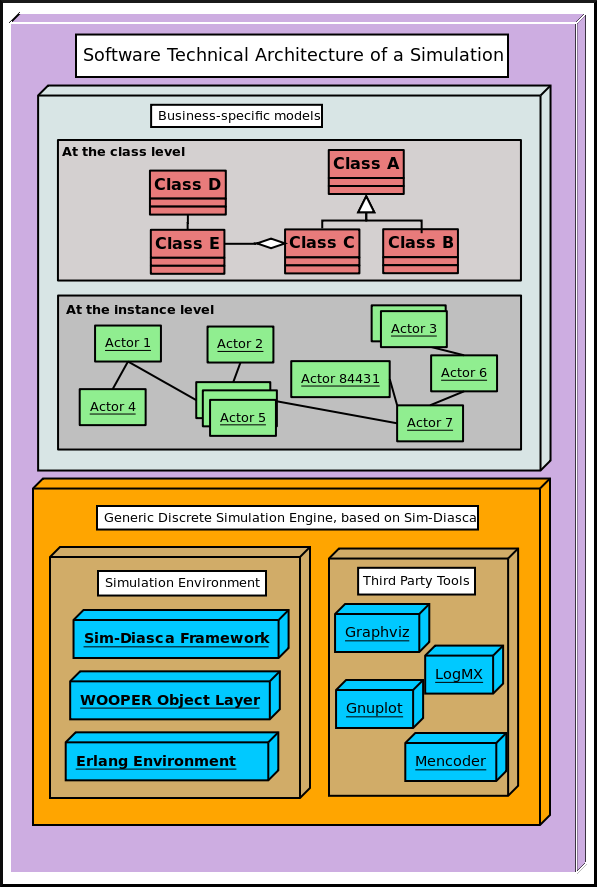
Therefore each element of the system can be represented by a set of models, of various nature and level of detail, results of the work of experts on various subjects, according to the following theoretical diagram:

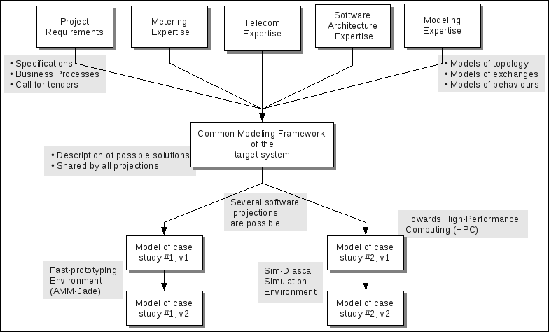
Different fields of expertise (notably functional and technical experts) have to define the simulation goals, metrics, and to work collaboratively on a set of common models, which form the modelling framework.

Once specified, the pool of models can be reused at will in the context of different experiments: these models can be assembled together and projected in various execution environments, with different purposes and level of detail.

Implementation Of Models

Uncoupling as much as possible models from implementations allows to reduce the dependency on a specific set of simulation tools, even though inevitably constraints remain.

In the case of the AMM project, two completely different simulation environments were developed, based on a common view of the system:

  • AMM-Jade, making use of the Jade multi-agent system, for fast prototyping purposes
  • Sim-Diasca, discussed here, making use of Erlang and of various custom-made layers, for finer modelling and HPC simulation purposes

These two threads of activity did not share any code but had a common approach to modelling.

In both cases, simulations operate on instances of models.

A model must be understood here in its wider sense: real system elements, such as meters or concentrators, are of course models, but abstract elements, like deployment policies or failure laws, can be models as well. Basically every stateful interacting simulation element should be a model, notably so that it can be correctly synchronised by the simulation engine.

A model can be seen roughly as a class in object-oriented programming (OOP).

Then each particular element of the simulation - say, a given meter - is an instance of a model - say, the AMM Meter model.

In agent-based simulations like the ones described here, all instances communicate only by message passing, i.e. shared (global) variables are not allowed. Added to code that is free from side-effects, seamless distribution of the processing becomes possible.

Unlike OOP though, the instances are not only made of a state and of code operating on them (methods): each and every instance also has its own thread of execution. All instances live their life concurrently, independently from the others. This is the concept of agents.

Relying on them is particularly appropriate here, as the reality we want to simulate is itself concurrent: in real life, the behaviour of all meters is concurrent indeed. Thus using concurrent software is a way of bridging the semantic gap between the real elements and their simulated counterparts, so that models can be expressed more easily and executed more efficiently.

Besides, these agents have to follow some conventions, some technical rules, to ensure that the aforementioned list of simulation properties can be met.

We finally call such a well-behaving agent a simulation actor, or simply an actor. The simulator can therefore be seen as a set of technical components that allow to operate on actors, notably in order to manage their scheduling and communication.

This topic is directly in relation with the issue of time management, which is discussed below.

A Short Overview of Simulation Services

From the point of view of a model writer, the main functional simulation services offered by Sim-Diasca are:

The main underlying technical simulation services are:

Sim-Diasca Time Management Explained

As already mentioned, the approach to the management of simulation time is most probably the key point of the design of a parallel, distributed simulation engine like the one discussed here.

There are several options to manage time, and, depending on the simulation properties that are needed, some methods are more appropriate than others.

Their main role is to uncouple the simulation time (i.e. the virtual time the model instances live in) from the wall-clock time (i.e. the actual time that we, users, experience), knowing that the powerful computing resources available thanks to a parallel and distributed context may only be used at the expense of some added complexity at the engine level.

Some General Technical Considerations First

In the context of interest here, a scheduler is a software component of a simulation engine that is specifically in charge of the management of the simulation time.

Its purpose is to preserve the simulation properties (e.g. uncoupling of the virtual time from the wall-clock one, respect of causality, management of concurrent events, management of stochastic behaviours, guarantee of total reproducibility, providing of some form of "ergodicity" - more on that later) while performing a correct evaluation of the model instances involved in that simulation.

It must induce as little constraint on the models as possible (e.g. in terms of fan-in, fan-out, look-ahead, etc.) and, as a bonus, it can evaluate them efficiently.

A scheduler can certainly be "ad hoc" (written in a per-simulation basis), but in the general cases we do not consider that this is a relevant option. Indeed much duplication of efforts would be involved, as such a scheduling feature would have to be repeatedly developed, from a simulation case to another, most probably in a very limited and limiting way.

Moreover ad hoc scheduling often results in static scheduling, where the modeller unwinds by himself the logic of the interaction of the various models federated by the simulation, and hardcodes it. We believe that much of the added value of a simulation is then lost in this case, the modeller removing many degrees of freedom and independence by emulating manually the role of a scheduler: in the general case, semantically the behaviour of a target system is best described as the natural by-product of several autonomous interacting entities, rather than as a predetermined series of events.

Preservation of Properties

Maintaining Causality

In the context of a distributed simulation, should no special mechanism be used, the propagation of simulated events would depend on the propagation of messages in the actual network of computing nodes, which offers no guarantee in terms of respective timing and therefore order of reception.

As the minimal example below [5] shows, a simulation cannot work correctly as such:

[5]The military setting is due to the fact their simulations have been ahead of civil ones for long.

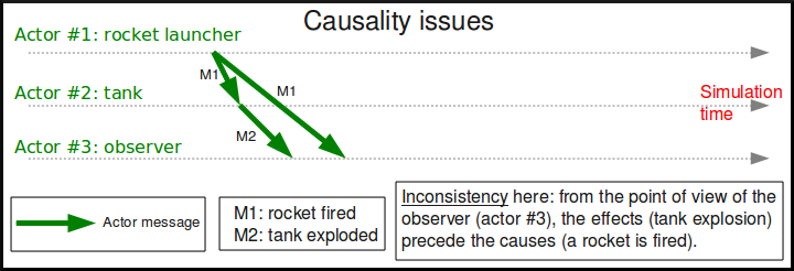
There are three simulation actors here, which are supposed to be instantiated each on a different computing node. Thus, when they communicate, they exchange messages over the network on which the distributed simulator is running.

Actor #1 is a rocket launcher that fires to actor #2, which is a tank. Thus actor #1 sends a message, M1, to all simulation actors that could be interested by this fact (including actor #2 and actor #3), to notify them of the rocket launch.

Here, in this technical context (computers and network), actor #2 (the tank) happens to receive M1 before actor #3 (the observer).

According to its model, the tank, when hit by a rocket, must explode. Therefore it sends a message (M2) to relevant actors (among which there is the observer), to notify them it exploded and that the corresponding technical actor is removed from the simulation.

The problem lies in the point of view of actor #3. Indeed in that case the observer received:

  1. M2, which told it that a tank exploded for no reason (unexpected behaviour)
  2. then M1, which tells it that a rocket was fired to a simulation actor that actually does not even exist

This situation makes absolutely no sense for this actor #3. At best, the model of the observer should detect the inconsistency and stop the simulation. At worse, the actor received incorrect inputs, and in turn injected incorrect outputs in a simulation that should not be trusted anymore.

The root of the problem is that here there is no guarantee that received messages will respect their timely constraints - whereas (at least in synchronous approaches) no return to the past shall be considered, however tempting.

This faulty behaviour would be all the more unfortunate that the incorrect outputs are likely to be indistinguishable from correct ones (i.e. they can go unnoticed in the simulation), distorting the results invisibly, a bit like a pocket calculator which would silently ignore parentheses, and would nevertheless output results that look correct, but are not.

Maintaining Reproducibility

Let's suppose for now we somehow managed to preserve causality. This does not imply that reproducibility is ensured.

Using the same example where actor #1 launches a rocket (sending the M1 message), actor #3 can in the meantime develop its own behaviour, which may imply this observer detected the tank. This can lead the observer notifying the tank, thus to its sending the M3 message.

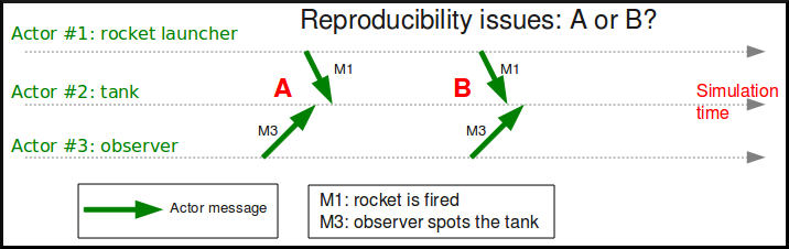
The point here is that there is no direct nor causal relationship between M1 and M3. These are truly concurrent events, they may actually happen in any order. Therefore concurrent events are not expected to be reordered by the mechanism used to maintain causality, since situations A and B are equally correct.

However, when the user runs twice exactly the same simulation, she most probably expects to obtain the same result [6]: here M1 should be received by actor #2 always before M3, or M3 always before M1, and the implicit race condition should not exist in that context.

[6]Otherwise she would not be able to interpret the consequences of a change in the simulation parameters unless she runs thousands of simulations to monitor macroscopic values only, instead of running two simulations (with and without the change) and comparing just the outcome of these two particular trajectories of the system.

In that case, causality is not enough, some additional measures have to be taken to obtain reproducibility as well.

With some time management approaches, once causality is restored, ensuring reproducibility is only a matter of enforcing an arbitrary order (i.e. which depends only on these messages, not in any way on the context) on concurrent events.

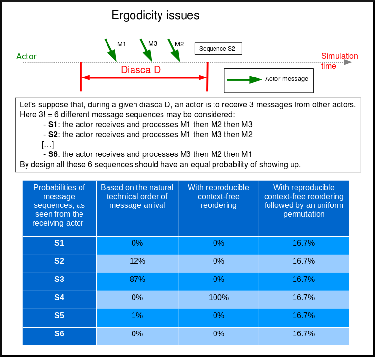
Allowing For Ergodicity

The context-free message reordering allows to recreate the arbitrary order we need to ensure reproducibility.

However the simulator should offer the possibility to go beyond this mechanism, otherwise "ergodicity" (a term we chose in reference to Monte-Carlo computations) cannot be achieved: in some cases we want all combinations of concurrent events to be able to occur, not only the ones that correspond to the arbitrary order we enforced.

Note

Just disabling the reproducibility mechanism would not be a solution: if no reordering at all was enabled, the natural sequence of concurrent events (which would then be dictated by the computing infrastructure) would not guarantee any ergodicity; some sequences of events would happen a lot more frequently than others, although they should not.

The best solution we know here is, in a time-stepped context, to let the reproducibility mechanism activated, but, in addition to the sorting into an arbitrary order, to perform then an uniform random shuffle: then we are able not only to recreate all licit combinations of events during a given simulation tick at the level of each actor, but also to ensure that all these combinations have exactly the same probability of showing up.

Approaches to Time Management

As far as we know, there are mainly four ways of managing time correctly, in a distributed context, in the context of a simulation in discrete time.

Approach A: use of a centralised queue of events

A unique centralised queue of simulation events is maintained, events are sorted chronologically, and processed one after the other.

Pros:

  • purely sequential, incredibly simple to implement

Cons:

  • splendid bottleneck, not able to scale at all, no concurrent processing generally feasible, distribution not really usable there; would be painfully slow on most platforms as soon as more than a few hundreds of models are involved

Approach B: use a time-stepped approach

The simulation time is chopped in intervals short enough to be able to consider the system as a whole as constant during a time step, and the simulator iterates through time-steps.

Pros:

  • still relatively simple to understand and implement
  • may allow for a massive, yet rather effective, parallelization of the evaluation of model instances
  • the simulation engine may be able to automatically jump over ticks that are identified as being necessarily idle, gaining most of the advantages of event-driven simulations
  • the resulting simulator can work in batch mode or in interactive mode with very small effort, and with no real loss regarding best achievable performance

Cons:

  • not strictly as simple as one could think, but doable (e.g. reordering of events must be managed, management of stochastic values must be properly thought of, induced latency may either add some constraints to the implementation of models or require a more complex approach to time management)
  • a value of the time step must be chosen appropriately (although we could imagine that advanced engines could determine it automatically, based on the needs expressed by each model)

Approach C: use a conservative event-driven approach

The simulation time will not advance until all model instances know for sure they will never receive a message from the past.

Pros:

  • efficient for systems with only few events occurring over long periods
  • there must be other advantages (other than the fact it is still a field of actual academic research) that I overlooked or that do not apply to the case discussed here

Cons:

  • complex algorithms are needed: it is proven that this mechanism, in the general case, leads to deadlocks. Thus a mechanism to detect them, and another one to overcome them, must be implemented
  • deadlock management and attempts of avoidance induce a lot of null (empty) messages to be exchanged to ensure that timestamps make progress, and this generally implies a significant waste of bandwidth (thus slowing down the whole simulation)

Approach D: use an optimistic event-driven approach

For each model instance (actor), simulation time will advance carelessly, i.e. disregarding the fact that other model instances might not have reached that point in time yet.

Obviously it may lead to desynchronised times across actors, but when such an actor receives a message from its past, it will rewind its logic and state in time and restart from that past. The problem is that it will likely have sent messages to other actors in-between, so it will have to send anti-messages that will lead to cascading rewinds and anti-messages...

Pros:

  • efficient in some very specific situations where actors tend to nevertheless advance spontaneously at the same pace, thus minimising the number of messages in the past received (not the case here, I think)
  • there must be other advantages (other than the fact it is still a field of actual academic research) that I overlooked or that do not apply to the case discussed here

Cons:

  • overcoming messages in the past implies developing a generic algorithm allowing for distributed roll-backs over a graph of model instances. This is one of the most complex algorithm I know and for sure I would not dare to implement and validate it, except maybe in a research-oriented project
  • even when correctly implemented, each simulation roll-back is likely to be a real performance killer

Sim-Diasca Time Management Algorithm

General Principles

Scheduling Approach

Sim-Diasca is based on approach B, i.e. it uses a synchronous (discrete time, time-stepped) algorithm for time management.

It has been deemed to be the most interesting trade-off between algorithmic complexity and scalability of the result. The manageable complexity of this approach allowed to bet on a rather advanced scheduler, featuring notably:

  • massive scalability, thanks to a fully parallel and distributed mode of operation yet with direct actor communication (i.e. inter-actor messages are never collected into any third-party agenda)
  • the ability to automatically jump over any number of idle ticks
  • the "zero time bias" feature, allowing to avoid any model-level latency in virtual time (causality solving does not make the simulation time drift)

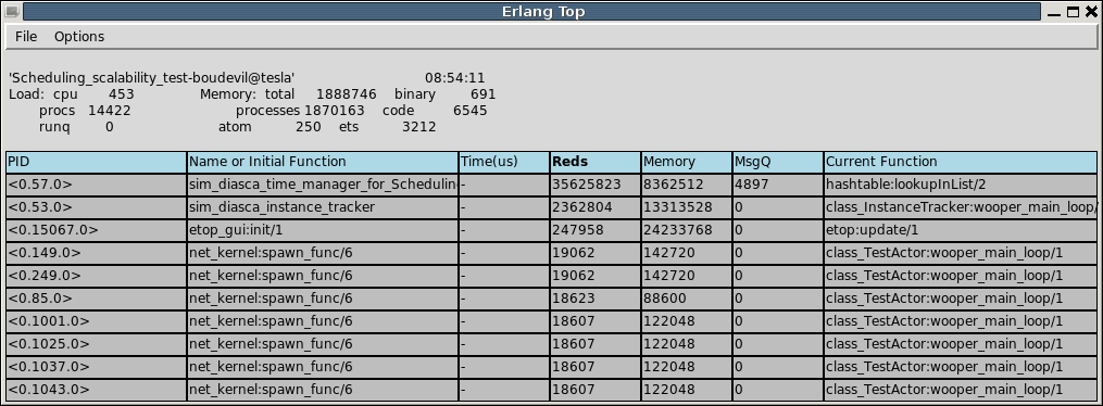
The simplicity of approach A was surely tempting, but when it evaluates one model instance at a time, the other approaches can potentially evaluate for example 35 millions of them in parallel. Fearless researchers might go for C or D. Industrial feedback about approach B was encouraging.

Architecture

In Sim-Diasca, the scheduling service is implemented thanks to an arbitrarily deep hierarchy of distributed time managers. Their role is to agree on the progress of simulation time and to allow model instances (actors) to be evaluated as much as possible in parallel.

More precisely, the simulation time is split according to a fundamental simulation frequency (e.g. 50 Hz, or vastly inferior ones for yearly temporalities) which defines the finest tick granularity (e.g. 20 milliseconds) on which model instances are free to develop their behaviour, however erratic and complex they may be.

Of course the time management service may then be able to perform "time-warp", i.e. to skip any series of ticks that it can determine as being idle.

However Sim-Diasca introduces a still finer, more flexible time management, as any scheduled tick will be automatically split by the engine in the minimal series of logical moments (named diascas) that is necessary to sort out causality [7]. This also allow for arbitrarily complex interactions while not inducing any time biases. And the point is that, inside a diasca, the engine is able to evaluate all scheduled model instances concurrently (in a parallel, possibly distributed way), and efficiently.

[7]A simulation timestamp can be represented as a (tick,diasca) pair: when a new tick T is scheduled, it will start at diasca zero, and the current diasca will be incremented as interactions are chained. More precisely, if the current timestamp is (T,D) and a then scheduled actor A1 performs an interaction, i.e. sends an inter-actor message M (a method, possibly with parameters) to an actor A2, then M will be sent by A1 and received by A2 during (T,D), yet A2 will process M (once automatically reordered with the other received messages, if any) only at (T,D+1), ensuring causality is met (effects happening strictly after their causes). A2, when executing the method corresponding to M, will be free to send in turn any number of actor messages to any actors; as soon as at least one message has been sent by one actor, (T,D+2) will be scheduled, and so on until no actor has a message to send. It will then be the last diasca for this tick T, and, if not terminated, the simulation will schedule the next tick according to the overall agenda, i.e. the next simulation timestamp will be (T',0), with T' > T.

Implementation

The message-based synchronisation is mostly implemented in the class_TimeManager module; the complementary part of the applicative protocol is in the class_Actor module, including the logic implementing the automatic message reordering (which happens to be fully concurrent).

Both can be found in the sim-diasca/src/core/src/scheduling directory.

Simplified Mode of Operation

A time step will be generally mentioned here as a simulation tick.

Sim-Diasca uses a special technical component - a process with a specific role - which is called the Time Manager and acts as the simulation scheduler.

It will be the sole controller of the overall simulation time. Once created, it is notably given:

  • a simulation start time, for example: Thursday, November 13, 2008 at 3:19:00 PM, from which the initial simulation tick will be deduced
  • an operating frequency, for example: 50 Hz, which means each virtual second will be split in 50 periods, with therefore a (constant) simulation tick whose duration - in virtual time - will be 1000/50 = 20 ms; this time step must be chosen appropriately, depending on the system to simulate [8]
  • an operating mode, i.e. batch or interactive
[8]Currently 50 Hz has been the highest frequency that was deemed useful for our application cases, knowing that this corresponded to a device scheduled by the 50 Hz electric power transmission.

In batch mode, the simulation will run as fast as possible, whereas in interactive mode, the simulator will be kept on par with the user (wall-clock) time. If the simulation fails to do so (i.e. if it cannot run fast enough), the user is notified of the scheduling failure, and the simulator tries to keep on track, on a best-effort basis.

Not depending on the operating mode, when started the Time Manager will always follow the same algorithm, shown below:

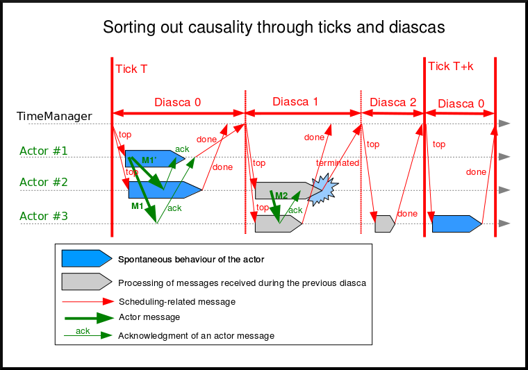
At the beginning of a new tick, the Time Manager will notify all subscribed simulation actors that a new tick began, thanks to a top message.

Each actor will then process all the actor messages it received during the last tick, reordered appropriately, as explained in the Maintaining Causality and Maintaining Reproducibility sections. This deferred message processing ensures the simulation time always progresses forward, which is a property that simplifies considerably the time management.

Processing these actor messages may imply state changes in that actor and/or the sending of actor messages to other actors.

Once all past messages have been processed, the actor will go on, and act according to its spontaneous behaviour. Then again, this may imply state changes in that actor and/or the sending of actor messages to other actors.

Finally, the actor reports to the time manager that it finished its simulation tick, thanks to a done message.

The key point is that all actors can go through these operations concurrently, i.e. there is no limit on the number of actors that can process their tick simultaneously.

Therefore each simulation tick will not last longer than needed, since the time manager will determine that the tick is over as soon as the last actor reported it has finished processing its tick.

More precisely, here each simulation tick will last no longer than the duration took by the actor needing the most time to process its tick, compared to a centralised approach where it would last as long as the sum of all the durations needed by each actor. This is a tremendous speed-up indeed.

Then the time manager will determine that the time for the next tick has come.

Actual Mode of Operation

For the sake of clarity, the previous description relied on quite a few simplifications, that are detailed here.

Distributed Mode Of Operation

The scheduling service has been presented as if it was centralised, which is not the case: it is actually fully distributed, based on a hierarchy of Time Manager instances.

Indeed they form a scheduling tree, each time manager being able to federate any number of child managers and of local actors. They recursively establish what is the next tick to schedule, each based on its own sub-hierarchy. The root time manager is then able to determine what is the next overall tick which is to be scheduled next (jumping then directly over idle ticks).

The current deployment setting is to assign exactly one time manager per computing host, and, for a lower latency, to make all time managers be direct children of the root one (thus the height of the default scheduling tree is one).

Other settings could have been imagined (balanced tree of computing hosts, one time manager per processor or even per core - rather than one per host, etc.).

Actual Fine-Grain Scheduling

The simulation time is discretised into fundamental time steps (ticks, which are positive, unbounded integers) of equal duration in virtual time (e.g. 10ms, for a simulation running at 100 Hz) that are increased monotonically.

From the user-specified simulation start date (e.g. Monday, March 10, 2014 at 3:15:36 PM), a simulation initial tick Tinitial is defined (e.g. Tinitial = 6311390400000).

Tick offsets can be used instead of absolute ticks; these offsets are defined as a difference between two ticks, and represent a duration (e.g. at 100Hz, Toffset=15000 will correspond to a duration of 2 minutes and 30 seconds in virtual time).

Internally, actors use mostly tick offsets defined relatively to the simulation initial tick.

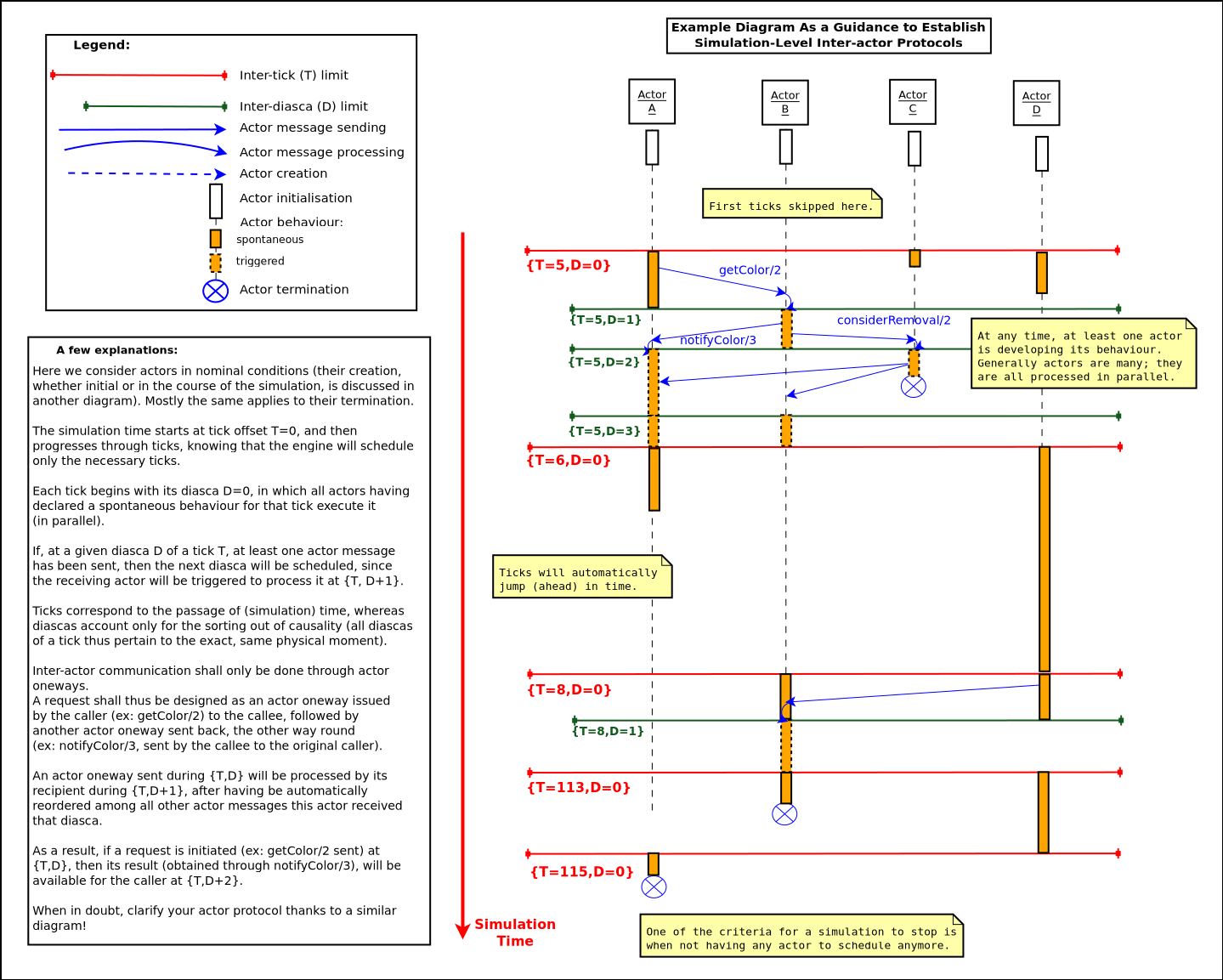
During a tick T, any number of logical moments (diascas, which are positive, unbounded integers) can elapse. Each tick starts at diasca D=0, and as many increasing diascas as needed are created to solve causality.

All diascas of a tick occur at the same simulation timestamp (which is this tick), they solely represent logical moments into this tick, linked by an "happen before" relationship: if two events E1 and E2 happen respectively at D1 and D2 (both at the tick T), and if D1 < D2, then D1 happened before D2.

So the full timestamp for an event is a Tick-Diasca pair, typically noted as {T,D}.

Diascas allows to manage causality despite parallelism: effects will always happen strictly later than their cause, i.e. at the very least on the diasca immediately following the one of the cause, if not in later diascas or even ticks, depending on the intended timing of the causal mechanism: causes can follow effects either immediately or after any specified duration in virtual time [9].

[9]Durations shall been specified by modellers regardless of a simulation frequency, in absolute terms (e.g. "6 minutes and 20 seconds"), rather than directly as a number of ticks: the engine is indeed able to convert the former to the latter at runtime, and to stop automatically if the conversion resulted in a rounding error higher than a threshold (either the default one, or a user-specified one for that duration). As much as possible, models should be uncoupled from the simulation frequency.

This is what happens when an actor A1 sends a message to an actor A2 at tick T, diasca D (i.e. at {T,D}). A2 will process this message at {T,D+1}. If needing to send back an answer, it may do it directly (while still at {T,D+1}), and A1 will be able to process it at {T,D+2}.

This allows immediate exchanges in virtual time (we are still at tick T - and A2 could have similarly triggered any number of third parties before answering to A1, simply resulting in an increase of the current diasca), while still being massively parallel and preserving causality and other expected simulation properties. Of course non-immediate exchanges are also easily done, since A2 may wait for any number of ticks before sending its answer to A1.

Consensus on the End of Tick

There must be a consensus between the actors to decide whether the current tick can be ended. One of the most effective way of obtaining that consensus is to rely on an arbitrator (the Time Manager) and to force the acknowledgement of all actor messages, from the recipient to the sender.

In the lack of such of an acknowledgement, if, at tick T, an actor A1 sent a message M to an actor A2, which is supposed here to have already finished its tick, and then sent immediately a done message to the Time Manager (i.e. without waiting for an acknowledgement from A2 and deferring its own end of tick), then there would exist a race condition for A2 between the message M and the top notification of the Time Manager for tick T+1.

There would exist no guarantee that M was received before the next top message, and therefore the M message could be wrongly interpreted by A2 as being sent from T+1 (and thus processed in T+2), whereas it should be processed one tick earlier.

This is the reason why, when an actor has finished its spontaneous behaviour, it will:

  • either end its tick immediately, if it did not send any actor message this tick
  • or wait to have received all pending acknowledgements corresponding to the actor messages it sent this tick, before ending its tick

Scheduling Cycle

Before interacting with others, each actor should register first to the time manager. This allows to synchronise that actor with the current tick and then notify it when the first next tick will occur.

At the other end of the scheduling cycle, an actor should be able to be withdrawn from the simulation, for any reason, including its removal decided by its model.

To do so, at the end of the tick, instead of sending to the Time Manager a done message, it will send a terminated message. Then the time manager will unregister that actor, and during the next tick it will send it its last top message, upon which the actor will be considered allowed to be de-allocated.

Note

The removal cannot be done during the tick where the actor sent its terminated message, as this actor might still receive messages from other actors that it will have to acknowledge, as explained in the previous section.

As for the management of the time manager itself, it can be started, suspended, resumed, stopped at will.

Criterion for Simulation Ending

Once started, a simulation must evaluate on which condition it should stop. This is usually based on a termination date (in virtual time), or when a model determines that an end condition is met.

Need for Higher-Level Actor Identifiers

When actors are created, usually the underlying software platform (e.g. the multi-agent system, the distribution back-end, the virtual machine, the broker, etc.) is able to associate to each actor a unique technical distributed identifier (e.g. a platform-specific process identifier, a networked address, etc.) which allows to send messages to this actor regardless of the location where it is instantiated.

However, as the reordering algorithms rely - at least partly - onto the senders of the messages to sort them, the technical distributed identifiers are not enough here.

Indeed, if the same simulation is run on different sets of computers, or simply if it runs on the same computers but with a load-balancer which takes into account the effective load of the computing nodes, then, from a run to another, the same logical actor may not be created on the same computer, and hence may have a different technical distributed identifier, which in turn will result in different re-orderings being enforced and, finally, different simulation outcomes to be produced, whereas for example reproducibility was wanted.

Therefore higher-level identifiers must be used, named here actor identifiers, managed so that their value will not depend on the technical infrastructure.

Their assignment is better managed if the load balancer take care of them.

On a side note, this actor identifier would allow to implement dynamic actor migration quite easily.

Load-balancing

Being able to rely on a load balancer to create actors over the distributed resources allows to run simulations more easily (no more hand-made dispatching of the actors over varying sets of computers) and, with an appropriate placing heuristic, more efficiently.

Moreover, as already mentioned, it is the natural place to assign actor identifiers.

The usual case is when multiple actors (e.g. deployment policies) need to create new actors simultaneously (at the same tick).

In any case the creating actors will rely on the engine-provided API (e.g. in class_Actor, for creations in the course of the simulation, create_actor/3 and create_placed_actor/4 shall be used), which will result in sending actor messages to the load balancer, which is itself a (purely passive) actor, scheduled by a time manager. These creation requests will be therefore reordered as usual, and processed one by one.

As for initial actor creations, still in class_Actor, different solutions exist as well:

  • create_initial_actor/{2,3}, for a basic creation with no specific placement
  • create_initial_placed_actor/{3,4}, for a creation based on a placement hint
  • create_initial_actors/{1,2}, for an efficient (batched and parallel) creation of a (potentially large) set of actors, possibly with placement hints

When the load balancer has to create an actor, it will first determine what is the best computing node on which the actor should be spawned. Then it will trigger the (synchronous and potentially remote) creation of that actor on that node, and specify what its Abstract Actor Identifier (AAI) will be (it is simply an integer counter, incremented at each actor creation).

As the operation is synchronous, for single creations the load balancer will wait for the actor until it has finished its first initialisation phase, which corresponds to the technical actor being up and ready, for example just having finished to execute its constructor.

Then the load balancer will have finished its role for that actor, once having stored the association between the technical identifier (PID) and the actor identifier (AAI), for later conversion requests (acting a bit like a naming service).

Actor - Time Manager Relationships

We have seen how a load balancer creates an actor and waits for its construction to be over.

During this phase, that actor will have to interact with its (local) time manager: first the actor will request the scheduling settings (e.g. what is the fundamental simulation frequency), then it will subscribe to its time manager (telling it how it is to be scheduled: step by step, passively, periodically, etc.), which will then answer by specifying all the necessary information for the actor to enter the simulation: what will be the current tick, whether the simulation mode targets reproducibility or ergodicity (in this latter case, an appropriate seed will be given to the actor), etc.

These exchanges will be based on direct (non-actor) messages, as their order does not matter and as they all take place during the same simulation tick, since the load balancer is itself a scheduled actor that will not terminate its tick as long as the actors have not finished their creation.

Actor Start-up Procedure

When models become increasingly complex, more often than not they cannot compute their behaviour and interact with other models directly, i.e. as soon as they have been synchronised with the time manager.

For instance, quite often models need some random variables to define their initial state. This is the case for example of low voltage meshes, which typically have to generate at random their supply points and their connectivity. As explained in the Actual Management of Randomness section, this cannot be done when the model is not synchronised yet with the time manager: reproducibility would not be ensured then.

Therefore the complete initialisation of such an actor cannot be achieved from its constructor only, and it needs an appropriate mechanism to determine at which point it is finally ready.

Moreover, as the start-up of an actor may itself depend on the start-up of other actors (e.g. the low-voltage mesh needs to wait also for its associated stochastic deployment policy to be ready, before being able in turn to live its life), Sim-Diasca provides a general mechanism that allows any actor to:

  • wait for any number of other actors to be ready
  • perform then some model-specific operations
  • declare itself ready, immediately or not, and notify all actors (if any) that were themselves waiting for that actor

The graph of waiting actors will be correctly managed as long as it remains acyclic.

This automatic coordinated start-up is directly available when inheriting from the Actor class.

Non-Termination Of Ticks

Some models can be incorrectly implemented. They may crash or never terminate, or fail to report they finished their tick.

The simulator will wait for them with no limit of time (as there is no a priori upper bound to the duration needed by a model to process its tick), but in batch mode a watchdog process is automatically triggered.

It will detect whenever the simulation is stalled and notify the user, telling her which are the guilty process(es), to help their debugging.

There could different reasons why an actor does not report its end of tick, notably:

  • its internal logic may be incorrectly implemented, resulting in that actor being unable to terminate properly (e.g. infinite loop)
  • the lingering actor (actor A) might be actually waiting for the acknowledgement from another actor (actor B) to which that actor A sent an actor message this tick

In the latter case the guilty process is in fact actor B, not actor A.

Both cases should be easy to interpret, as the time manager will gently nudge the lingering actors, ask them what they are doing, and then output a complete diagnosis, both in the console and in the simulation traces:

Simulation currently stalled at tick #3168318240271, waiting for following actor(s): [<0.50.0>,<0.57.0>].
Current tick not ended yet because:
 + actor <0.50.0> is waiting for an acknowledgement from [<0.1.0>]
 + actor <0.57.0> is waiting for an acknowledgement from [<0.1.0>,<0.38.0>]

Now moreover the engine is able most of the time to also specify the name of the actors that are involved, for a better diagnosis.

Distributed Execution In Practise

For the scenario test case to be able to run a simulation on a set of computing nodes from the user node, that node must be able to trigger the appropriate Sim-Diasca daemon on each computing node.

To do so, a SSH connection is established and the appropriate daemon is run. The recommended set-up is to be able to run a password-less connection to the computing nodes. This involves the prior dispatching of a private key is these nodes, and the use of the corresponding public key by the user host.

See, in the Sim-Diasca Installation Guide, the Enabling The Distributed Mode Of Operation section for the corresponding technical procedure.

Model Development

All generic mechanisms discussed here (actor subscription, synchronisation, reordering and acknowledgement of actor messages, removal, waiting to be ready, etc.) have been abstracted out and implemented in a built-in Actor class, to further ease the development of models.

They should therefore inherit from that class and, as a consequence, they just have to focus on their behavioural logic.

Of Times And Durations

User Time Versus Simulation Time

Regarding simulation timing, basically in batch mode the actual user time (i.e. wall-clock time) is fully ignored, and the simulation engine handles only timestamps expressed in virtual time, also known as simulation time. The objective there is to evaluate model instances as fast as possible, regardless of the wall-clock time.

In interactive mode, the engine still bases all its computations on virtual time, but it forces the virtual time to match the real time by slowing down the former as much as needed to keep it on par with the latter (possibly making use of a scale factor).

Therefore the engine mostly takes care of simulation time, regardless of any actual duration measured in user time (except for technical time-outs).

Units of Virtual Time Versus Simulation Ticks

Virtual time can be expressed according to various forms (e.g. a full time and date), but the canonical one is the tick, a quantum of virtual time whose duration is set by the simulation user (see the tick_duration field of the simulation_settings record). For example the duration (in virtual time) of each tick can be set to 20ms to define a simulation running at 50Hz.

Ticks are absolute ticks (the number of ticks corresponding to the duration, initially evaluated in gregorian seconds, between year 0 and the specified date and time), ans as such are often larger integers.

For better clarity and performances, the simulation engine makes heavy use of tick offsets, which correspond to the number of ticks between the simulation initial date (by default a simulation starts on Saturday, January 1st, 2000 at midnight, in virtual time) and the specified timestamp. So #4000 designates a tick offset of 4000 ticks.

Note that one can sometimes see expressions like this happened at tick #123. The dash character (#) implies that this must be actually understood as a tick offset, not as an (absolute) tick.

Models should define all durations in terms of (non-tick) time units, as actual, plain durations (e.g. 15 virtual seconds), rather than directly in ticks or tick offsets (like #143232). Indeed these former durations are absolute, context-less, whereas the corresponding number of simulation ticks depends on the simulation frequency: one surely does not want to have to update all the timings used in all models as soon as the overall simulation frequency has been modified.

So the recommended approach for models (implemented in child classes of class_Actor) is to define, first, durations in time units (e.g. 15s), and then only to convert them, as soon as an actor is created (i.e. at simulation-time), into a corresponding number of ticks (e.g. at 2Hz, 15s becomes 30 ticks) thanks to the class_Actor:convert_seconds_to_ticks/{2,3} helper functions [10].

[10]A corresponding method (convertSecondsToTicks/2) could be used instead, however this method has virtually no chance of being overloaded any day, so using the helper functions is not a problem.

This class_Actor:convert_seconds_to_ticks/2 function converts a duration into a non-null integer number of ticks, therefore a rounding is performed, and the returned tick count is at least one (i.e. never null), in order to prevent that a future action ends up being planned for the current tick instead of being in the future, as then this action would never be triggered.

Otherwise, for example a model could specify a short duration that, if run with lower simulation frequencies, could be round off to zero. Then an actor could behave that way:

  • at tick #147: set action tick to current tick (147) + converted duration (0) thus to #147; declaring then its end of tick
  • next tick: #148, execute:
case CurrentTick of

  ActionTick ->

      do_action();
      ...

However CurrentTick would be 148 or higher, never matching ActionTick=147, thus the corresponding action would never be triggered.

Ticks Versus Tick Offsets

Ticks are absolute ticks (thus, generally, huge integers), whereas tick offsets are defined relatively to the absolute tick corresponding to the start of the simulation.

Of course both are in virtual time only (i.e. in simulation time).

Tick offsets are used as much as possible, for clarity and also to improve performances: unless the simulation runs for a long time or with an high frequency, tick offsets generally fit into a native integer of the computing host. If not, Erlang will transparently expand them into infinite integers, which however incur some overhead.

So, in the Sim-Diasca internals, everything is based on tick offsets, and:

  • when needing absolute ticks, the engine just adds to the target offset the initial tick of the simulation
  • when needing a duration in simulation time, the engine just converts tick offsets into (virtual, floating-point) seconds
  • when needing a date in simulation time, the engine just converts a number of seconds into a proper gregorian date
Starting Times

By default when a simulation is run, it starts at a fixed initial date, in virtual time [11], i.e. Friday, January 1, 2010, at midnight. Of course this default date is generally to be set explicitly by the simulation case, for example thanks to the setInitialTick/2 or setInitialSimulationDate/3 methods. These timings are the one of the simulation as a whole.

[11]This arbitrary date was previously set to the current real time, so that the simulations started from the present time of the user. However we could then have variations in the results despite reproducible simulations, if using models depending on the absolute (virtual) date (e.g. in the simulation, each 1st of April, do something).

Simulations will always start at tick offset #0 (constant offset against a possibly user-defined absolute tick) and diasca 0.

On the actor side, each instance has its own starting_time attribute, which records at which global overall simulation tick it was synchronized to the simulation.

Implementing an Actor

Each model must inherit, directly or not, from the actor class (class_Actor). As a consequence, its constructor has to call the one of at least one mother class.

Each constructor should start by calling the constructors of each direct parent class, preferably in the order in which they were specified; a good practice is to place the model-specific code of the constructor after the call to these constructors (not before, not between them).

An actor determines its own scheduling by calling oneways [12] helper functions offered by the engine (they are defined in the class_Actor module):

  • addSpontaneousTick/2 and addSpontaneousTicks/2, to declare additional ticks at which this instance requires to develop a future spontaneous behaviour (at their diasca 0)
  • withdrawnSpontaneousTick/2 and withdrawnSpontaneousTicks/2, to withdraw ticks that were previously declared for a spontaneous behaviour but are not wanted anymore
  • declareTermination/1, to trigger the termination of this actor
[12]Note that corresponding helper functions are also defined (e.g. class_Actor:add_spontaneous_tick/2); they can be called directly if the user is sure that he will never need to override their oneway counterpart.

An actor is to call these helper functions from its actSpontaneous/1 oneway or any of its actor oneways. This includes its onFirstDiasca/2 actor oneway, which is called as soon as this actor joined the simulation, so that it can define at start-up what it intends to do next, possibly directly at this very diasca (no need for example to wait for the first next tick).

Even if actors are evaluated in parallel, the code of each actor is purely sequential (as any other Erlang process). Hence writing a behaviour of an actor is usually quite straightforward, as it is mostly a matter of:

  • updating the internal state of that actor, based on the changes operated on the value of its attributes (which is an immediate operation)
  • sending actor message(s) to other actors (whose processing will happen at the next diasca)

On each tick the engine will automatically instantiate as many diascas as needed, based on the past sending of actor messages and on the management of the life cycle of the instances.

So the model writer should consider diascas to be opaque values that just represent the "happened before" relationship, to account for causality; thanks to these logical moments which occur during the same slot of simulated time, effects always happen strictly after their causes.

As a consequence, the model writer should not base a behaviour onto a specific diasca (e.g. "at diasca 7, do this"); the model should send information to other instances or request updates from them (in both cases thanks to other messages) instead.

So, for example, if an actor asks another for a piece for information, it should just expect that, in a later diasca (or even tick, depending on the timeliness of the interaction), the target actor will send it a message back with this information.

The point is that if the model-level protocol implies that a target actor is expected to send back an answer, it must do so, but at any later, unspecified time; not necessarily exactly two diascas after the request was sent: we are in the context of asynchronous message passing.

This allows for example an actor to forward the request to another, to fetch information from other actors, or simply to wait the duration needed (in virtual time) to account for any modelled processing time for that request (e.g. "travelling from A to B shall last for 17 minutes").

When actor decides it is to leave the simulation and be deleted, it has to ensure that:

  • it has withdrawn all the future spontaneous ticks it may have already declared
  • it calls its declareTermination/{1,2} oneway (or the class_Actor:declare_termination/{1,2} helper function)

The actor must ensure that no other actor will ever try to interact with it once it will have terminated, possibly using its deferred termination procedure to notify these actors that from now they should "forget" it.

Please refer to the Sim-Diasca Developer Guide for more information.

Latest Enhancements

These evolutions have been implemented for the 2.0.x versions of Sim-Diasca, starting from 2009.

Distributed Time Manager

The Time Manager was described as a centralised actor, but actually, for increased performances, the time management service is fully distributed, thanks to a hierarchy of time managers.

By default there is exactly one time manager per computing host, federating in an Erlang node all cores of all its processors and evaluating all the actors that are local to this host (and only them).

One of these time managers is selected (by the deployment manager) as the root time manager, to be the one in charge of the control of the virtual time. The other time managers are then its direct children (so the height of the scheduling tree is by default equal to 1).

Other kinds of trees could be chosen: they might be unbalanced, have a different heights (e.g. to account for multiple clusters/processors/cores), etc., as shown in the physical diagram below:

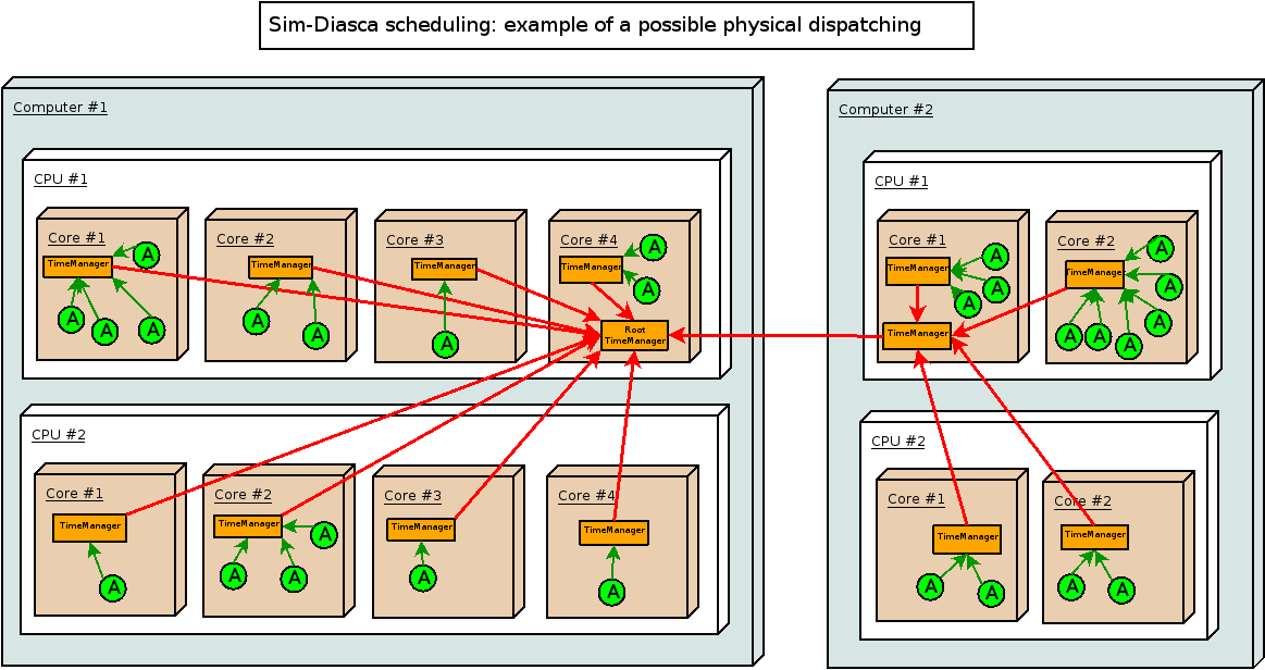
The overall objective is to better make use of the computing architecture and also to minimize the induced latency, which is of paramount importance for synchronous simulations (we want to be able to go through potentially short and numerous time-steps as fast as possible).

Two protocols are involved in terms of scheduling exchanges, as shown in the logical diagram:

  • one for higher-level synchronisation, between time managers
  • another for lower-level actor scheduling, between a local time manager and the actors it drives

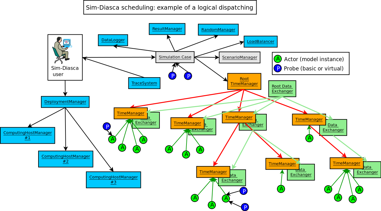
Of course there will be many more actors than displayed on the diagram created on each computing node (typically dozens of thousands of them), therefore a lot of scheduling messages will be exchanged between these actors and their local time manager instance.

The point is that these (potentially numerous) messages will incur as little overhead as possible, since they will be exchanged inside the same computing node: only very few scheduling messages will have to cross the node boundaries, i.e. to be conveyed by the bandwidth-constrained network. We trade the number of messages (more numerous then) for their network cost, which is certainly a good operation.

The load balancer has to be an actor as well (the only special one, created at start-up), since, when the simulation is running, it must be able to enforce a consistent order in the actor creations, which, inside a time step, implies the use of the same message reordering as for other actors.

In the special case of the simulation set-up, during which the initial state of the target system is to be defined, the initial actors have to be created, before the simulation clock is started. Only one process (generally, directly the one corresponding to the simulation case being run; otherwise the one of a scenario) is expected to create these initial actors. Therefore there is no reordering issues here [13].

[13]However race conditions must be avoided there (between creations and also with the simulation start), this is why all initial creations are by design synchronous.

Advanced Scheduling

Each model may have its own temporality (e.g. a climate model should imply a reactivity a lot lower than the one of an ant), and the most reactive models somehow dictate the fundamental frequency of the simulation.

A synchronous simulation must then be able to rely on a fundamental frequency as high as needed for the most reactive models, yet designed so that the other models, sometimes based on time-scales many orders of magnitude larger, can be still efficiently evaluated; scalability-wise, scheduling all actors at all ticks is clearly not an option (short of wasting huge simulation resources).

Moreover most models could not simply accommodate a sub-frequency of their choice (e.g. being run at 2 Hz where the fundamental frequency is 100 Hz): their behaviour is not even periodic, as in the general case it may be fully erratic (e.g. determined from one scheduling to the next) or passive (only triggered by incoming actor messages).

So Sim-Diasca offers not only a full control on the scheduling of models, with the possibility of declaring or withdrawing ticks for their spontaneous behaviours, but also can evaluate model instances in a rather efficient way: this is done fully in parallel, only the relevant actors are scheduled, and jumps over any idle determined to be idle are automatically performed (based on a consensus established by the time managers onto the next virtual time of interest; if running in batch, non-interactive, mode).

With this approach, and despite the synchronous simulation context (i.e. the use of a fixed, constant time step), the constraints applied to models are very close to the ones associated to event-driven simulations: the difference between these two approaches is then blurred, and we have here the best of both worlds (expressiveness and performance).

Finally, models ought to rely as much as possible on durations (in virtual time) that are expressed in absolute units (e.g. "I will wait for 2 hours and a half") instead of in a frequency-dependent way (e.g. "I will wait for 147 ticks"): the conversion is done automatically at runtime by the engine (with a mechanism to handle acceptable thresholds in terms of relative errors due to the conversions), and the model specifications can be defined as independently as possible from the fundamental frequency chosen by the simulation case.

Zero-Time Bias Modelling

Despite such a tick-level flexibility, by default time biases cannot be avoided whenever solving causality over ticks. Indeed, if, to ensure effects can only happen strictly after their causes, actor messages are evaluated on the tick immediately following the one of their sending, then for example all request/response exchange patterns will induce a two-tick latency.

This is unfortunate, as this latency is not wanted (not present in the models), and moreover depends on the fundamental frequency of the simulation. No immediate interaction can happen then, and if the target of a request needs to get information from other actors, the latency will still increase, with no upper limit.

To solve this significant modelling constraint, a zero-time bias feature has been added to Sim-Diasca (in 2012), introducing the notion of diascas, which are numbered logical moments inside a tick. A tick is then actually composed of an unbounded series of diascas, the first one (diasca 0) corresponding to the time when all actors having planned a spontaneous behaviour are to develop it. This may include the sending of actor messages, which in turn leads to the creation of the next diasca: each actor having received a message at a diasca will then be scheduled accordingly at the next diasca, and may then send messages, and so on.

As a consequence, the advanced scheduling, once enriched with diascas, is able to adapt to any model-level scheduling, and to support all interactions, either immediate or delayed, involving any communication chain underneath, in a causality-free way, and still in a massively parallel manner.

This flexibility regarding virtual time with no biases opens in turn new outlooks, for example to run in parallel, with Sim-Diasca, models that are written in the context of a mere sequential simulator, or, possibly, to go towards hybrid simulations, where some models are ruled by continuous equations yet are to be integrated with the discrete part of the simulation, helped by a numerical solver and further integration efforts.

How Virtual Time is Managed

Virtual Time Versus Real Time

In batch mode, the time of the simulation (a.k.a. virtual time) is fully decorrelated from the user, wall-clock time: the engine will run as fast as possible, but will take as long as needed to fully evaluate simulated events. As a consequence, depending on the computer resources that are used, the resulting simulation might be faster or slower than real-time.

In interactive mode, provided that the hardware is able to run the simulation faster than the real time (possibly once a user-specified scaling factor has been applied), the engine will perform the necessary waiting so that the virtual time stays on par with the real time, allowing for possible third-party interactions with the simulation (actual devices, humans in the loop, etc.).

Quantification & Timings

The virtual time is quantised, i.e. chunked into slices of equal durations (this is why Sim-Diasca is a discrete synchronous simulation engine). These periods are called simulation ticks (often shorten as ticks here).

For example, if the user specifies a tick duration of 20ms, then all durations will be multiples of 20ms (possibly 0ms - instant actions are supported) and the simulation will run at 50Hz.

Note that, for the models to be as much as possible uncoupled from the simulation frequency, they should express their timings in terms of actual "absolute" durations (e.g. 100ms), rather than in terms of a number of ticks (e.g. 5 ticks, at 50Hz).

This way, changing the simulation frequency (e.g. setting it to 100Hz) will not imply that all models need to have their internal timing settings updated accordingly; indeed the engine is able to convert at runtime such actual durations into the relevant number of ticks, and will automatically ensure that the relative quantification error that is then induced stays below a threshold (either the default one or a user-defined one). If the quantification error is too high, the simulation will just report it and stop.

Spontaneous Behaviours & Triggered Actions

At its creation (whether initial or in the course of the simulation), each actor is scheduled once and is able to tell the engine at which tick (if any) it plans to develop its next spontaneous behaviour.

The engine (actually, the root time manager) is then able to know for each new tick whether it should be scheduled (this will happen iff at least one actor planned a spontaneous action for that tick). This knowledge will then allow the simulation to automatically jump over ticks that are known to be idle (i.e. with no actor to schedule). This feautre allows such a synchronous engine to provide features that are quite similar to the ones provided by asynchronous engines.

However, such a simulation would be useless if the actors could not interact with other actors: during a tick, any actor is able to trigger actions on any other actor.

Causality & Diasca

To ensure, even in a parallel and/or distributed setting, that no cause can happen after its effects, the model instances can only communicate through the exchange of actor messages.

These messages can be seen as method calls which are properly intercepted, reordered and actually triggered by the engine.

For that the notion of diasca is introduced: each tick is evaluated as a series of diascas (starting at diasca D=0), each of them being a logical moment inside that tick.

The purpose of diascas is to split each tick so that the consequence of an event (an actor message is sent at diasca D) happens at the next diasca (the actor message is processed by its recipient at diasca D+1).

These triggered actions may in turn result in new actor messages being sent, resulting in as many diascas as needed (D+2, D+3, etc.) being instantiated. The current tick will terminate only when no more diascas are requested, i.e. when there is no more immediate action declared. Then the next tick will be scheduled, and will start from diasca 0 again.

As such, diascas do not correspond to any specific duration within a tick (which is by design the finest observable simulated duration): their purpose is just to allow to determine that some events happen before others, i.e. to maintain causality.

Next Steps: Time Generalization

We plan to support the following time-related generalizations:

  • to provide more flexibility and granularity, ticks could be of a parametrised type, i.e. a user-decided, simulation-specific type (e.g. they could be floats instead of being integers), provided that they respect a (simple) contract specified by the engine; see class_TimeManager:tick() for more details
  • to allow for recursive, imbricated/nested actors (actors containing, or being made of actors) and time refinement, diascas could be tuples (e.g. {17,5,0}, {17,5,1}, etc. being between {17,5} and {17,6}, themselves being between 17 and 18); see class_TimeManager:diasca() for more details

In-Depth: Scheduling Implementation

The simulations being distributed, the time management is itself distributed.

For that, a hierarchy of time managers is defined. Any scheduling tree can be defined, knowing that by default there will be one time manager per computing host (thus federating all cores of all local processors), and that they will form a flat tree: the engine will select an appropriate host for the root time manager (which will the sole manager of virtual time), and all others will be direct children of it.

Each time manager will schedule all the actors that are local to its node. This way, the large majority of scheduling messages will remain local to an Erlang node (i.e. potentially millions), and only the inter-manager ones (i.e. a few) will be exchanged over the network.

At the beginning of a tick T that is to be scheduled (as idle ticks will be jumped over automatically), the root time manager will trigger a {beginTimeManagerTick,T} to all its direct children, which will forward it recursively to their own children, if any. Then each time manager will send a {beginTick,T} messages to all its local actors that were scheduled for a spontaneous action this tick.

They will develop then each (in parallel) their spontaneous behaviour, being implicitly at diasca D0=0 for that tick T. Each actor can then update its state and/or send inter-actor messages.

Sending an actor message in asynchronous (not blocking) and results in the recipient actor storing the corresponding method call for a deferred execution (at the next diasca), and to send a {scheduleTrigger,T,D} message to its own local time manager (which might already have terminated its diasca) so that it knows that this actor will have then to be triggered. Once its manager acknowledged that message (needed to prevent race conditions) thanks to a `trigger_planned message, the recipient actor can then directly acknowledge to the sending actor that its message was processed, thanks to a {acknowledgeActorMessage,T,D,...} message.

Once a scheduled actor will have completed its spontaneous actions and received all acknowledgements for the actor messages it sent this diasca, it will notify its time manager by sending it a {spontaneous_behaviour_completed,T,D0,DiascaOutcome} message, where DiascaOutcome is no_diasca_requested if it did not send any actor message, or next_diasca_needed otherwise.

Once all actors scheduled by a time manager complete a given diasca, this manager will report to its direct parent manager (if any) whether or not a new diasca is needed, by sending it a {childManagerSpontaneousActionsCompleted,...} message specifying, among other information, either no_diasca_requested or next_diasca_needed.

As soon as at least one actor among all the scheduled actors for this diasca sent at least one actor message, the root time manager is notified that a new diasca D (still for tick T) is needed. Time managers will then recursively receive a {beginTimeManagerDiasca,T,D} message and in turn will send, to the actors they schedule that received during the previous diasca an actor message, a {beginDiasca,T,D} message.

Each of these triggered actors will then reorder all the messages it received during the previous diasca, and then process them in turn, possibly changing its state and/or sending new actor messages, which will in turn lead to a new diasca being needed, etc.

Once such a triggered actor completed its diasca, it sends back to its time manager a {diasca_completed,T,D} message. Once all the local actors triggered for this diasca did so, their time manager sends a {child_manager_diasca_completed,...} message specifying, among other information, either no_diasca_requested or next_diasca_needed to its own direct parent manager.

Sim-Diasca Management of Probabilistic Laws

Principles

Quite often models rely on the use of stochastic variables, i.e. variables from which values can be drawn according to their associated Probability Density Function.

Such variables - respecting a given probabilistic law - are very useful to model the behaviours of simulation actors.

For example, in terms of reliability, an approach may be to define per-equipment average constants like the Mean Time To Failure (MTTF) and the Mean Time To Repair [14] (MTTR), and to express reliability models thanks to stochastic laws parameterised by these constants (for the previous example, these would be two exponential laws).

[14]MTTR is also known as Mean Time To Recovery.

Stochastic variables are also very useful when generating variations on a theme, in the context of the simulation of a large number of instances of a given case.

For example, when wanting to simulate a wide range of different low-voltage meshes, one can either:

  • load a set of externally-defined descriptions of real meshes coming from the field (should such descriptions be available, accurate and numerous enough)
  • or, more easily, one can generate these different meshes according to some probabilistic rules, which would give, for example, the number of supply points of a given mesh, depending on its profile (e.g. rural, urban, etc.), so that the pool of generated meshes follows the real-life statistics

The objective here is therefore to provide model developers with all the facilities needed to easily specify and implement stochastic models, in full compliance with the aforementioned simulation properties. This involves a little more than that:

Built-in Random Distributions

Although any probabilistic distribution (i.e. probability density) may be defined and added to the framework, Sim-Diasca provides some built-in distributions, listed below, that are among the most common, notably in the domain of reliability studies.

In technical terms, they are defined in Myriad's random_utils, and used to be gathered in the RandomManager; nowadays using one's PDF is considerably simpler, as any actor can directly define any number of random laws and simply draw samples from them. Alternatively, a model may derive from the StochasticActor class in order to more conveniently define and access to its random laws.

Uniform Law

This "white noise" generator will draw values into a user-parameterised range, all samples having an equal probability of being chosen.

When placing a Sim-Diasca probe at the output of a RandomManager set to deliver a uniform law, we have the following result:

By setting the appropriate flag, Sim-Diasca can also be configured to use a uniform generator of superior quality, which was designed for cryptography.

This uniform distribution is often the basis to generate in turn more complex distributions.

Exponential Law

This distribution, defined by a single parameter, lambda, leads to the following result:

This distribution is directly generated by Sim-Diasca from the previous white noise source.

Gaussian Law

Two parameters, mu, the mean value, et sigma, the variance (whose positive square root is the standard deviation), define the Gaussian law [15].

[15]It is also known as the normal law.

This results in the following curve:

The Sim-Diasca white noise generator is used to generate this Gaussian law as well.

Extra Reliability-Oriented Laws

A total of about 20 random laws are supported (uniform, exponential, gaussian, Gamma, Weibull, Gumbell, etc.; this includes all distributions defined from here), some with a few variations (with integer samples rather than floating-point ones, yiedling only positive values, etc.), each defined based on a set of parameters.

Even if some laws (uniform, exponential, gaussian) may be obtained by a direct use of the per-actor embedded random generator, most are computed through inverse transform sampling (precisely the alias method, once the PDF has been discretised).

These laws are typically considered by the Python Reliability library as candidate blueprints that may fit actual data: such libraries will attempt to determine the best choice in terms of function and associated parameters to match as closely as possible the input data.

Note

Another option, should the history/feedback be deep enough, would be, instead of fitting it and discretising the obtained function, to use that feedback directly as the PDF from which samples are to be drawn.

User-Specified Random Distributions

Non-uniform, arbitrarily-defined probability density functions are supported.

For that, refer, in the random_utils module, to the generate_random_state_from/2, get_sample_from/1 and get_sample_from/2 functions, and to the corresponding Myriad section.

Actual Management of Randomness

Random Generators

At the core of most implementations, one relies on a random generator, which usually outputs floating-point values uniformly distributed between 0.0 and 1.0.

For a better stochastic management, the engine does not rely anymore on the basic random module of Erlang; it may operate instead with the crypto module (if available and enabled), otherwise it will default on the newer rand module, which offers various algorithms, including:

  • exsplus: Xorshift116+, 58 bits precision and period of 2^116-1 (state uses 320 bytes on 64-bit platforms)
  • exs64: Xorshift64*, 64 bits precision and a period of 2^64-1 (state of 336 bytes on 64-bit platforms)
  • exs1024: Xorshift1024*, 64 bits precision and a period of 2^1024-1 (state of 856 bytes on 64-bit platforms)

Unless overridden (see random_utils.erl), the algorithm used by the engine is exsplus.

Based on a uniform random value in [0.0,1.0], one can generate uniform values in any other range, and values that respect all kinds of non-uniform laws (like the Gaussian one).

However a question still remains: how many instances of random generators should we use?

Mode Of Operation

Random generators usually have a state, which is initialised with a seed - either set by default, or specifically given.

From a seed a series of random numbers can be generated, and as such it can be reproduced identically, as long as the same seed is used.

The trouble comes from the fact that, during any given logical moment (diasca), multiple simulation actors may require - and therefore request from a random generator - any number of values complying to any number of probabilistic laws, each parameterised as wished, in any order. And of course we do not want to loose the reproducibility of simulations because of that.

Initially the engine was relying on a limited number of centralised random manager instances (possibly even just one), each used by a (potentially large) set of model instances.

Each of these model instances would then interact with its random manager(s) in a consistent manner, through actor messages to preserve simulation properties.

Such an approach induces many constraints, like the additional synchronisation and diasca creation involved (hence significant runtime overhead), a more complex model-level logic to request and wait for these values, etc.

Detailed: Why Centralised Random Managers are Evil

(please feel free to skip this section if not having historical curiosity)

The most obvious approach for stochastic management is to have actors require the random values they need to a centralised random manager.

This solution is simple, but has some pitfalls, particularly if the engine does not provide a concept of "logical moments", i.e. diascas here.

A central objective is of course not to break reproducibility. Indeed, without any specific measure, actors would request their value to the centralised random manager during the execution of their tick, with no particular order enforced between requests, since they would be concurrent in that context.

Therefore, if, thanks to the seeding, they would indeed consume collectively always the same random series, the values of this series would be differently dispatched among actors, depending on the chronological order of reception of their requests by the random manager.

A solution is to have the random manager become a simulator actor as well. Then it would be appropriately synchronised by the mechanisms provided by the time manager, and stochastic actors would thus behave correctly and in a reproducible way.

There is an issue there nevertheless. Indeed, if the model of an actor required that actor to use a random value at a given tick N, then to have that value the actor would have to send a request during this tick to the random manager, which would process that request during the next tick (i.e. N+1) and send back the determined value to the requesting actor, which would in turn be able to process it no sooner than the next tick (N+2).

Therefore this would induce by default an unwanted 2-tick latency each time an actor would require a random value, whereas the model would not tell us so. As some actors can consume at least one value per tick, the system cannot work as is.

Moreover, not all actors are able to anticipate on their needs of random values, and, in the cases where it would be possible, doing so would make their implementation a lot more complex than needed.

Hence, before diascas were introduced, a generic solution had been designed instead - which would manage transparently these needs, i.e. with no impact on the writing of models.

The solution consists on having each actor that uses stochastic variables define, for each one of them, not only which distribution law with which settings should be used, but also an upper bound to the number of values following that law that may be drawn during any single tick, for this actor and this distribution.

Such an upper bound should be possible to define for most if not all models and, if ever the upper bound was incorrectly evaluated (i.e. if it was set to a too small value, leading to an exhaustion of the corresponding random buffer), then at simulation time the issue would be detected and the simulation would stop. Then the upper-bound could just be set to a higher value, and the simulation be run again.

With these information, the generic stochastic actor (a Sim-Diasca built-in) was able to transparently cache full lists of random variables obtained from the (centralised) random manager, and to manage their refilling appropriately in the background, so that the corresponding random values could be always obtained with zero latency by an actor.

Thus the implementation of models was considerably simplified, since they can be developed as if they could rely on local infinite random sources, which additionally would not raise issues about reproducibility.

This was coming at the expense of extra diascas being instantiated (forcing models to manage them and hitting the runtime performances) and a few extra constraints.

For example, apart from the already mentioned constraint regarding the upper bound in terms of the number of drawn samples, some stochastic actors need random variables whose probabilistic distributions can change during a simulation. For example, if a meter determines its connectivity by drawing, even with equal probability, a given number of meters out of its functional upstream meters, this translates into a uniform law whose range can change at each tick (depending on how many upstream meters are functional); this is a problem for this kind of approaches based on transparent buffering.

The specialised generic actor, the Stochastic Actor - which can be reused at will by all stochastic models to simplify their development - used to rely on this mechanism. Since then, we opted for a simpler and more efficient system, explained below.

Current Mode of Operation

A more flexible approach has been finally retained: each model instance embeds its own, private, random generator (to which it can readily and freely access without constraint), which is seeded appropriately (on a reproducible manner, each actor having its own, specific seed) when that actor is created.

This removes all drawbacks previously mentioned, at the expense of:

  • a more complex actor creation done by the load balancer (in charge of a parallel yet proper seeding - itself based on its own random generator)
  • an increased memory footprint of the stochastic actors, as each must store the state of its random generator (typically ranging from 32 bytes to a few kilobytes)

Thanks to this on-creation seeding, reproducibility is ensured, and stochastic actors are able to interact with their embedded random generator with no further synchronisation effort, i.e. with no delay nor message (actor or not).

Randomness Pitfalls

All model instances are automatically correctly seeded, so all probabilistic laws can be readily used from them with no effort.

However, in some cases (typically for initialisation purposes, in the simulation case) it may be useful to rely on basic processes, WOOPER or not (i.e. not actors), and some of them might have to be stochastic (e.g. when generating a given road network following specific constraints). These helper processes should have their random source explicitly seeded (using random_utils:start_random_source/{1,3} for that), otherwise a non-constant seed will be assigned to each of them, and it will break reproducibility.

Another potential cause of issue is the change of a random source: if not explicitly seeded, some of them will default on a constant seed (e.g. random) while others not (e.g. rand, the current default source).

As a result, all non-actor processes having to generate, directly or not, random values shall be explicitly seeded, typically thanks to:

random_utils:start_random_source( default_seed )

Sim-Diasca Management of Simulation Inputs

Principles

A simulation is defined primarily by its simulation case, which shall specify the simulation inputs.

These inputs are mostly:

  • the technical settings, like the various simulation, deployment and load balancing settings (see the corresponding records to properly specify these inputs)
  • the initial state of the simulation, i.e. what are the initial actors and scenarios, and in which state they shall be when the simulation begins

Requirements

The initial state of the simulation is by far the most challenging input to manage. In simple cases, it can be seen as a series of (synchronous) creations of initial instances (actors or scenarios, no difference from the engine's point of view), which can be done:

  • either programmatically - directly from the simulation case or from a scenario (in both cases typically thanks to a series of class_Actor:create_initial_actor/{2,3} calls, with the relevant parameters in terms of model construction)
  • or based on initialisation data, read from any kind of information stream (typically user-specified initialisation files)

Initialisation may not be straightforward, notably because actors may have to know others, forming a directed graph that may comprise cycles.

A simple example would be when two actors (A and B) have to know each other initially. This initial state cannot be created in one pass as, when the first actor is created (let's say: A), the second (B) does not even exist yet - so A will have to be created as if it were alone, and must be notified afterwards that it is to know B - once B will have been created as well [16].

[16]B then could be fully created in one pass, since A is existing at this point. However, to preserve symmetry and homogeneity, and avoid being associated to a A instance that is partly initialised (it does not know B yet), probably B should be created in two passes, exactly as A.

Furthermore, in order to designate instances, most simulation projects tend to rely on identifier conventions of their own, that are specific to these simulations and may be of approximately any datatype.

For example some projects will rely on numerical instance identifiers (e.g. 1275411), other may use names (e.g. 1600 Pennsylvania Ave NW, Washington, DC 2050012, United State) while some simulations could rely on more complex data structures (e.g. (12,3.0,45), whatever this may mean).

Qualities of an input management system include:

  • allowing most kinds of user-specific instance identifiers
  • managing its own, private identifiers transparently for the user
  • being able to sort out all cyclic dependencies
  • not preventing at least some sort of efficient distributed mode of operation afterwards, notably with regard to smart placement and load-balancing
  • relying on an expressive, yet compact and human-readable, form to specify the initial instances
  • managing this initialisation data as much as possible in parallel

Creation of the Initial State of the Simulation

How to Create Initial Instances Programmatically

This is the easiest, yet most limited, approach. No external identifier needs to be involved here.

If wanting to create two instances that have to know each other, one may use, possibly directly from the simulation case:

A = class_Actor:create_initial_actor( class_Foo, [ Xa, Ya ] ),
B = class_Actor:create_initial_actor( class_Bar, [ Xb, Yb, Zb ],
   "My placement hint" ),

A ! { declareBar, B, self() },
B ! { declareFoo, A, self() },

bar_declared = test_receive(),
foo_declared = test_receive(),

[...]

A few remarks here:

  • A and B are PIDs
  • this mutual recognition requires a specific method to be added in both classes (namely declare{Foo,Bar}/2)
  • one can guess that the declare{Foo,Bar}/2 methods exposed here are requests (even if no particular result had to be returned), for synchronicity reasons (otherwise there could be a race condition between these messages and the ones related to the start of the simulation); this is why we have to receive the *_declared messages from the simulation case
  • we can see that here A will be created using default placement policy, when B will be created by the load balancer according to the specified hint: when created programmatically, all instances specifying the same placement hint will be created on the same computing node (as chosen by the load balancer)

How to Use Initialisation Data to Create Initial Actors

Specifying the Data Source

The user shall call, either directly from the simulation case or from a scenario: sim_diasca:create_initial_instances/1 [17]

[17]We use instances, as they may be actors or scenarios.

or use the initialisation_files field of the simulation_settings (see soda_loading_test.erl for an example).

In both cases we expect a list of filenames to be specified, each being a path (absolute, or relative to the directory from which Sim-Diasca was launched) to a file containing initialisation data of interest.

Each of them should be a text file (whose name is arbitrary, but we recommend using the .init file extension; for example: my-case-instances.init), containing a series of lines, either:

  • blank
  • or containing a comment
  • or containing a creation specification, ending with a dot

Any line may have any number of leading and/or trailing whitespaces.

Each non-empty line that is not a comment is to create an instance, hence shall specify the class name and actual construction parameters that correspond to this instance.

See the soda-instances.init file (in the soda-test mock simulator) for a full example.

Regarding Actor Identifiers

To better integrate into most architectures, Sim-Diasca manages two kinds of identifiers for actor instances created from data:

  • external ones, i.e. the arbitrary identifiers that are provided by the user, which are often simulation-specific
  • internal ones, i.e. identifiers that are managed internally by the engine, and which are mostly transparent for the user

External identifiers can be arbitrary strings, which are processed as are (no attempt of checking, parsing or enforcing any convention on their content is made there) [18].

[18]We could even imagine that these identifiers be of any type, however this would offer little practical interest.

The internal identifiers are simply the PID of the corresponding instances.

Thus the engine takes care of letting the user rely on any convention, while maintaining a two-way translation scheme to benefit from the best of both worlds.

Format of a Line for Basic Creation

Such a line is made of a pair, whose first element is the class (as an atom) of the instance to create and whose second element is a list containing its construction parameters, that may be approximately any Erlang terms [19].

[19]We will see below that actually only tuples whose first element is the user_id atom are not accepted as actual initialisation data, since, in this context, they would be ambiguous.

A simple line, designated as a "creation clause", could then be:

{class_Foo,["Hello world!",1.4]}.

One can see this data-based initialisation as a simple counterpart to this programmatic form:

class_Actor:create_initial_actor(class_Foo,["Hello world!",1.4])

Such a data-based initialisation allows expressing all creations of initial instances - except the ones that start interlinked and thus that must rely on some sort of (user-defined) instance identifiers.

A basic creation can also be performed with an additional parameter, which is a placement hint (which can be any term). This tells the load balancer to create all instances that are specified with the same placement hint on the same computing node.

Such a creation clause can then be, if using an atom as hint:

{class_Foo,["Hello world!",1.4],my_placement_hint}.

The corresponding programmatic form being then:

class_Actor:create_initial_placed_actor(class_Foo,
  ["Hello world!",1.4],my_placement_hint)

Format of a Line Specifying a User Identifier

The following syntax allows, in addition to the aforementioned creation, to define and associate a specific user-provided identifier to that newly created instance.

We can see that the same basic creation pair as before is now prefixed by its user identifier and an arrow:

"My first instance" <- {class_Foo,["Hello world!",1.4]}.

As a consequence, the engine will see the "My first instance" string as a user identifier associated to the PID of the corresponding class_Foo initial instance that will be created.

The user identifiers are arbitrary strings, except that they should not contain any double quote (") character (to simplify their parsing).

For the engine, defining a user identifier results in selecting a related placement of the upcoming instance. Hence no placement hint can be specified with this form.

Of course defining identifiers would be useless if they could not be used afterwards.

Format of a Line Making Use of a User Identifier

Such a line would be for example:

{class_Bar,[an_atom,3,{user_id,"My first instance"},7]}.

We can see here that the user identifier previously defined for the class_Foo instance (i.e. My first instance) will be used in order to create the class_Bar instance, so that the latter can know the former (i.e. have its PID) from its start (on its creation).

When referenced (as opposed to being defined), user identifiers are to be tagged thanks to a user_id pair. For example {user_id,"My first instance"} is to be specified, instead of a mere "My first instance" (which would be interpreted as any random string).

Otherwise simple parameter strings and user identifiers could not be discriminated properly; the user_id atom is thus reserved for such use.

No user identifier being defined here, a placement hint can also be specified. For example as a string (here, "Milky Way"):

{class_Dalek,[true,{user_id,"EXTERMINATE"}],"Milky Way"}.

Format of a Line in the General Case

Often a given instance will reference some others (i.e. rely on their user identifier) and have its own user identifier defined, like in:

"John" <- {class_Beatle,[{user_id,"Paul"},{user_id,"George"}]}.

Here John will know from the start Paul and George, and later in the initialisation phase any Ringo could know John as well, using {user_id,"John"} for that.

As always, a user identifier being defined here, no placement hint can be specified.

More Information About Placement Hints

We can see that no placement hint could be specified in the creation lines above, as they defined a user identifier.

Indeed, with data-based initialisations, placement derives naturally from user identifiers:

  • if a user identifier is specified (e.g. "My Foo" <- {class_Foo,[...]}), then this identifier ("My Foo") will be used as a placement hint
  • if no user identifier is specified:
    • if a placement hint is specified, then it will be used directly
    • if no placement hint is specified either:
      • if no user identifier is referenced either (e.g. {class_Foo,["Hello world!",1.4]}.), then the corresponding instance will be placed according to the default policy of the load balancer
      • if at least one user identifier is referenced (e.g. {class_Foo,[2,{user_id,"AA"},0.0,{user_id,"BB"}, my_atom]}.), then the corresponding instance will be placed according to the first user identifier found when parsing the construction parameters; so, in this example, this class_Foo instance would be created on the same computing node on which the instance designated by user identifier "AA" will be

This allows an automatic, implicit placement of instances which by design are likely to interact.

Comments

An initialisation file may also contain comments. They have to be on a dedicated line, starting with the character %. Then the full line is ignored.

Empty Lines

There are ignored.

Inner Workings Explained

The initialisation data is read and, in parallel, is parsed and checked by a set of creator processes (one per core of the user host).

One instance is created per read creation line (provided it is neither blank nor a comment), and the engine ensures that a hosting process is available for each instance referenced in that creation line: any user identifier referenced before being defined will result in a blank process being spawned on the relevant computing node (determined solely from this user identifier); this process will embody the corresponding instance, once its definition will be processed.

The PID of each of these created processes is recorded in a translation table, so that user identifiers can be related to these processes.

Despite the arbitrary creation order induced by parallelism, the engine takes care of assigning reproducible AAIs and random seeds.

In the meantime the read initialisation terms are transformed, replacing each {user_id,UserIdentifier} pair (of course these information can be arbitrarily nested in any kind of data-structure, discovered at runtime) by the corresponding PID (that is either already pre-spawned or created at this moment), and the corresponding instances are initialised (their constructor being called with the relevant, transformed construction parameters).

Each user identifier must be defined exactly once; any user identifier:

  • referenced to, but never defined, results in an error
  • defined more than once results in an error

A user identifier that is defined but never referenced is not considered as an error.

When the parsing of a creation line fails, a detailed context is given (with the faulty line verbatim, the file name and line number, and an interpretation of the error).

The JSON syntax could have been used here (for example relying on jiffy or on jsx), but it would not be nearly as compact and adequate as the custom syntax proposed here.

Model Initialisation

One must understand that the indirection level provided by user identifiers allows the engine to create initial instances in any order (regardless on any potentially cyclic dependency), thus at full speed, in parallel, with no possible deadlock and while preserving total reproducibility.

This system is designed not to add any constraint onto the actors or scenarios; this however implies that, once a given instance is constructed, any other instance it references (through user_id) may or may not be already constructed; nevertheless its PID is already available and given to the referencing instance, and thus once constructed it will be able to answer any pending message(s) transparently.

The model developer of course should ensure that the deadlocks spared by this instance creation system are not re-introduced by their initialisation logic.

This should not be a real problem, as the trickiest issue, the exchange of references, is already solved by design here.

Sim-Diasca Management of Simulation Outputs

Principles

A simulator allows to run virtual experiments, involving input parameters and models, and producing corresponding outputs, a subset of it being tagged as the actual results awaited by the user. Some post-processing can then be later applied to these results, which are usually rather raw by-products.

The overall goal is to obtain, from known facts and thanks the simulations, new knowledge that was not necessarily anticipated.

Indeed, in the same way as one may rely on a (hopefully validated) oracle or a gyroscope, the outcome of a simulation cannot be really precisely foreseen (otherwise it would be plain useless):

Managing The Outputs

In the general case, simulation outputs comprise results, traces, user interface data, etc. We focus below on the simulation results.

General Mode of Operation

Sim-Diasca offers a fully concurrent support for simulation results (from their generation to their retrieval), so that they are efficiently produced (only the relevant ones, and in a massively parallel way) and automatically returned back to the user in its launching directory, knowing that on a distributed context the output data is by design scattered across the various networked computing nodes.

For that, if and if only the simulation finishes successfully, a directory specific to that simulation run (based on simulation name, time and date, user and a rather unique identifier [20]) is created in the current directory (i.e. the directory from which make My_Case_run was executed) of the user node; this result directory bears a name like:

Sim-Diasca_My_Case-on-2015-12-10-at-10h-05m-59s-by-boudevil-1f793a6ba507

Results of interest are automatically transferred there (otherwise one would have to log in on each and every computing node [21] to select and retrieve these results by hand).

[20]An effort is made to generate names for result directories that can hardly collide, as for example in the context of parametric studies a launcher script may trigger, from the same location and on behalf of the same user, the execution of multiple simulation cases per second. The identifier mentioned here is the SII, detailed in the What is the Simulation Instance Identifier? section of the Sim-Diasca Developer Guide.
[21]All computing nodes uses a temporary directory for their work, which includes extracting the deployment archive to access to the simulation input data and code, and storing locally the results being produced. The name of this directory (by default placed under /tmp/) is forged in order to be reasonably unique (e.g. sim-diasca-My_Case-boudevil-2015-12-10-at-10h-05m-59s-1f793a6ba507), to avoid clashes between simulations that would run concurrently on shared computing hosts.

Results are handled by:

  • the overall Result Manager (a class_ResultManager singleton, automatically created at deployment time on the user node), which keeps track of results and drive them
  • Result producers (all class_ResultProducer instances, like probes, either basic or datalogger-based), which provide support to declare, aggregate and send their results

Following mode of operation allows to handle results:

  1. the simulation user specifies initially, in the simulation case, what are the results he is interested in, thanks to a Result Specification (detailed below)
  2. the result manager checks this specification, and precomputes what will be needed to discriminate between wanted and unwanted simulation results
  3. when the creation of result producers (typically probes instantiated from models or scenarios) is considered (either initially or at simulation-time), it is declared automatically to the result manager, which is then able to tell whether a given result producer is wanted or not (then only the necessary producers will be created and fed); this allows a given model to support any number of probes, and to enable only the relevant ones on a per-simulation case basis
  4. in the course of the simulation, result producers gather sample data, performing immediate or deferred writes (their volume usually exceeds the capacities of the overall distributed RAM), potentially terminating at any time and then performing operations on these data (e.g. generating plots from them)
  5. when (if) the simulation ends successfully, the result manager automatically requests the relevant results from all relevant producers, and copy them in the result directory (more precisely, it generates them only if appropriate, like in the case of plots, and send them in a compressed from over the network, to the user node)

Result Specification

Which results are wanted is generally specified directly from the simulation case, among the simulation settings.

The selection is based on the names of the result producers to enable, since it is the only way the user can refer to them a priori (e.g. of course no PID can be statically anticipated in the simulation case).

In the result specification, a simulation case may require:

  • a binary selection: either all results are wanted or none of them
  • a type-based selection: either the results corresponding to plain probes or to virtual ones (i.e. based on the data-logger) are wanted
  • a finer pattern-based selection: only results whose name matches at least one targeted pattern, and none of the blacklisted patterns, are to be selected (most general case)

Patterns are to be expressed according to the Perl Compatible Regular Expressions conventions, or PCRE for short.

For more information on the pattern format, see the re module.

The detailed supported syntax is specified in the sim-diasca/src/core/src/scheduling/class_TimeManager.hrl header file; see the result_specification field of the simulation_settings record. Examples can be found in the cases available in the mock-simulators directory.

Relying on these simulation settings allows to define which results are expected statically, which is fine for most uses. However, under some circumstances, it may be convenient to set or modify the result specification dynamically (e.g. if it is difficult to anticipate on the name of a probe or whether it is actually wanted).

Thus result specification can be also modified at simulation-time, thanks to method calls (see the {add,remove,set}{Targeted,Blacklisted}Pattern*/2 methods of class_ResultManager).

Early Disabling of Results

All results could be generated in all cases, and only be retrieved if requested.

However a better approach could be to collect data samples and process them (e.g. in graphical plots) only if needed.

A still better approach is needed: as the result manager is able to tell directly whether a result is wanted, it will be able to disable unwanted results from the start, i.e. reject any attempt of creating a result producer (e.g. a probe) whose results are not wanted by the user.

As a consequence, a classical, model-level probe may be created thanks to the class_Probe:declare_result_probe/6 static method, which will return either the PID of this newly created probe (if the name of that probe is acknowledged as a wanted result by the result manager), or the non_wanted_probe atom.

Then the class_Probe:send_data/3 method can be called as often as needed by the model in order to potentially feed that probe with relevant sample data (the fact that this probe may not be enabled being then transparently managed).

Result Generation

Often, many models are able to define various probes, and the corresponding number of instances is huge.

A large number of result producers may therefore exist, even after having selected (thanks to the result specification) only a subset of them.

The consequence is that the parallel, distributed result generation cannot be triggered as a whole, lest the most loaded computing nodes will simply crash (e.g. RAM exhausted).

The result manager therefore implements a flow control mechanism, ensuring that all possible computing nodes work at full speed, while not being too much overloaded. Basically, at any time, up to twice as many generations are requested as there are cores on a given computing host. Any generation completion yields the requesting of another pending one (if any).

Post-Processing the Results

Some approaches and tools can be used to transform results into knowledge. This involves generally synthesising the vast amount of data into a few relevant statistics or indicators.

The post-processing to be done depends significantly on the specific problem being studied. Currently, except probe reports, Sim-Diasca outputs mainly time series, letting the user feed these raw data to the suitable tools, on a domain-specific way.

Interpreting the Outcome

Once the right questions have been properly formalised, this step is probably, with the validation part, the trickiest part of a simulation work: what are the lessons learned, and to which extent can we trust them?

Providing detailed guidelines would be beyond the scope of this document. Here are nevertheless a few hints.

Identifying Reasons For Observed Phenomena

Finding actual causes is seldom straightforward:

Having Reasonable Expectations

A simulation is not the silver bullet that will ask the right questions on the user's behalf and answer them with infinite accuracy:

Simulation being a rather expensive and time-consuming mode of evaluation, it should be used on carefully selected cases that cannot be solved satisfactorily thanks to other methods, like comparison with actual systems, expert assessments, coarse spreadsheet-based studies, etc.

Even in that case, a few well-selected metrics must be defined, that must be both helpful to the user and solvable by the simulation.

Extrapolating Results, Really?

Unless it has been proven separately, one cannot arbitrarily reduce the problem size and expect that a small-scale experiment will still provide reliable insights about a real-sized system: reductionism cannot be applied blindly.

This is why the scalability of a simulation engine is a key property: whenever smaller-scale experiments cannot be safely attempted (the general case), it offers a better chance of capturing the reality.

Indeed extrapolating becomes too often a wild guess:

In most cases, approaches based on extrapolations are hardly sustainable:

Sharing the Findings With the Intended Audience

The lessons learned thanks to the simulation must be synthesised appropriately, with proper wording for the targeted public, so that the conclusions are sufficiently emphasized to be well-understood:

Concerns must be correctly shared among the people involved, with appropriate common metrics and goals:

Making Good Use of the New Knowledge

It is certainly out of the scope of this document, but simulations may generate new knowledge, which must be carefully leveraged, lest it worsens the situation:

Sim-Diasca Reliability

Context

The simulations of complex systems tend to be of a larger scale, and may last (at least in wall-clock time) very long.

Numerous computing hosts will then be involved in such simulations and, even if each of the cores of these hosts boasts a high MTBF, their number will imply that, if waiting for long enough, any proportion of them will fail [22]. Not to mention that there will be as well network issues, transient or not.

[22]The MTBF of a petascale system is not expected to exceed 10 hours, while reports about some Bluegene supercomputers suggests a MTBF of a few days (of course loosing a core may not take down the whole machine, but would "only" make the job(s) relying on that core fail themselves.

As a result, without a specific mechanism for resilience, some demanding simulations would be (especially in future uses) unlikely to complete at all.

This is why a k-crash resilience feature has been added to the Sim-Diasca engine, starting from its 2.2.0 version.

Note

Many loosely related features have been improved or added since the introduction of resilience system, while some of them would have required to update accordingly that system.

One should thus consider that, as long as the resilience mechanisms below have not been updated, the resilience feature as a whole is currently not available.

A Tunable Resilience Service

Now, at start-up, the user of a simulation is able to specify, among the simulation settings (see, in class_DeploymentManager.hrl, the crash_resilience field of the deployment_settings record), what is the required level of resilience of the simulation with regard to the loss of computing hosts in its course:

  • either none is required (the default mode), in which case the simulation will crash as soon as a computing host is deemed lost (while, on the other hand, no resilience-induced overhead will exist in this case)
  • or a positive integer k is specified, which designates the maximum number of simultaneous losses of computing hosts that the simulation will be able to overcome (a safety net which, of course, will imply some corresponding overhead - it is actually quite reasonable)

For example, if k=3, then as long as up to 3 computing hosts fail at the same time during a simulation, it will be nevertheless able to resist and continue after a short (bounded) automatic rollback in simulation-time.

This will include starting again from the last simulation snapshot (established automatically at the latest wall-clock simulation milestone, if any was met), converting back the states of simulation agents, actors and result producers (probes) which had been then serialised, re-dispatching (load-balancing-wise), re-creating, updating and linking the corresponding processes, before making the simulation time progress again from that milestone.

There is no upper bound in the number of total losses of computing hosts in the simulation that can be overcome, provided that at any time the k threshold is not exceeded [23] and that the remaining hosts are collectively able to sustain the resulting load.

This last point implies that the resources of a fault-tolerant simulation must exceed the strict needs of a simulation offering no resilience. For example, if N homogeneous hosts are assigned to a k-resilient simulation, then the user must ensure that the simulation can indeed fit at the very least in N - k computing hosts, otherwise there is no point in requesting such a resilience.

[23]Currently, hosts that departed the simulation cannot join back. As a consequence, the remaining ones must be able to cope with the load. Therefore the simulation user ought to allocate a little more resources than strictly necessary initially, to compensate for the sum of all later losses, as they will not be redeemed. The extra hosts introduced in this case behave as spare ones, except that they do not remain idle until a host crashes: they participate to the simulation from its very start, to further smooth the computing load.

Note that this resilience applies only to the random "workers", i.e. to the average computing hosts. For example, if the host of the root time manager is lost, the simulation will crash, regardless of the value of k. Depending on the optional services that are enabled (e.g. performance tracker, data-logger, data-exchanger, etc.) other single points of failures may be introduced, as they tend to be deployed on different hosts (trade-off between load-balancing and resilience) [24]. Currently, depending on the aforementioned enabled services, very few single points of failure remain (typically up to three, compared to a total number of computing hosts that may exceed several hundreds, if not thousands in the near future).

[24]Most, if not all, services could be made resilient; we simply started with the key ones. As we are able to store most of the reproducible simulation state and reconstruct the purely technical, transient information, a given simulation might even survive the loss of all its computing nodes, and restart later from a blank state, just based on its serialisation data.

Similarly, should a long-enough network split happen, the k threshold may be immediately reached. If running on production mode, extended time-outs should provide a first level of safety.

Currently no support is offered for hosts that would join in the course of the simulation to compensate for previous losses (for example if being rebooted after a watchdog time-out): usually dynamic additions are not in line with the practice of cluster job managers (it is simpler and more efficient to directly use a larger number of nodes upfront).

Besides the resilience level (i.e., the number k), a (possibly user-defined) serialisation period will apply. It corresponds to the lower bound in terms of (wall-clock [25]) duration between two serialisations (default duration is two hours).

[25]Since hardware and software faults are ruled by wall-clock time; simulation time may flow in a very different manner.

This serialisation activity will run even before the simulation is started, so that even simulations needing a long time to recreate their initial situation benefit from some protection (typically such a serialisation will then happen at the very first evaluated diasca).

Finally, we ensured that this serialisation activity does not introduce a non-negligible latency (whether activated or not) - but, of course, once the regular serialisation is triggered, the whole simulation is bound to be stalled for some time (even if it is done in an almost fully parallel, distributed way). As a consequence, the resilience feature is only compatible with the batch mode of operation (i.e. not with the interactive one).

Mode of Operation

Preparing for any later recovery

Let's suppose that N computing hosts are assigned to a simulation having to exhibit a k-crash resiliency.

This resilience service is implemented internally by first establishing a "k-map", which determines, for each of the N hosts, which of the k other hosts it backs-up and, reciprocally, which hosts back it up.

For example, if N=6, hosts may be [a,b,c,d,e,f], and the k-map could then be, for a requested resilience level of k=5:

For a resilience level of 5, result is: k-map for 6 nodes:
+ for node a:
 - securing nodes [b,c,d,e,f]
 - being secured by nodes [f,e,d,c,b]

+ for node b:
 - securing nodes [c,d,e,f,a]
 - being secured by nodes [f,e,d,c,a]

+ for node c:
 - securing nodes [d,e,f,a,b]
 - being secured by nodes [f,e,d,b,a]

+ for node d:
 - securing nodes [e,f,a,b,c]
 - being secured by nodes [f,e,c,b,a]

+ for node e:
 - securing nodes [f,a,b,c,d]
 - being secured by nodes [f,d,c,b,a]

+ for node f:
 - securing nodes [a,b,c,d,e]
 - being secured by nodes [e,d,c,b,a]

This example corresponds to, graphically (see class_Resilience_test.erl):

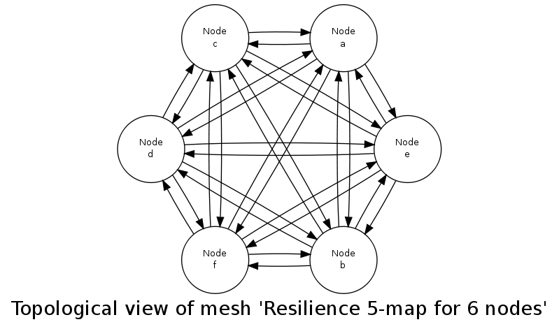
Of course this resilience feature is typically to be used with a far larger number of nodes; even with a slight increase, like in:

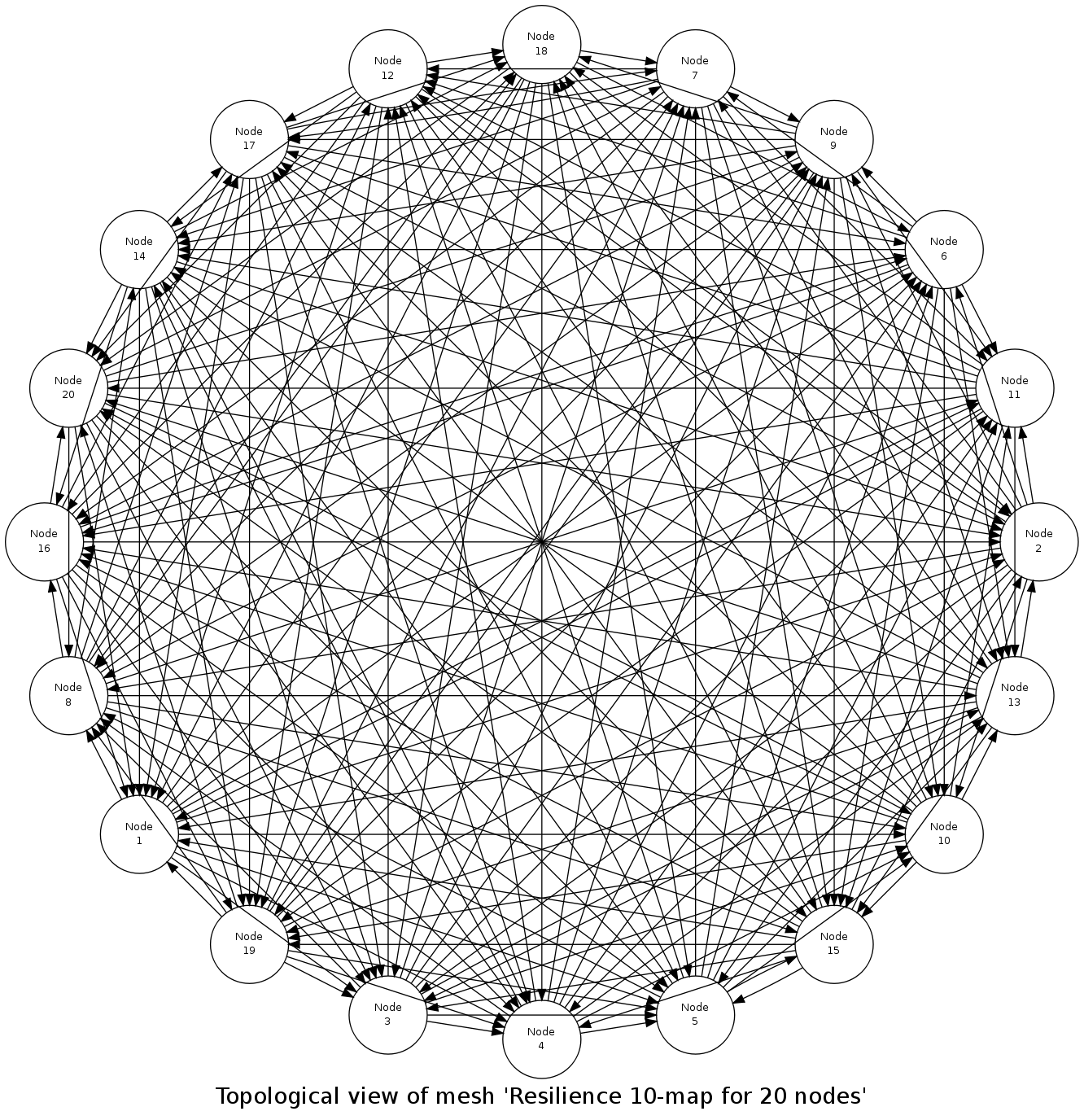
we see that any central point in the process would become very quickly a massive bottleneck.

This is why the actual work (both for serialisation and deserialisation tasks) is done in a purely distributed way, and exchanges are done in a peer-to-peer fashion, using the fastest available I/O for that [26], while the bulk of the data-intensive local work is mostly done in parallel (taking advantages of all local cores).

[26]This includes tuned file writing and reading, operating on stripped-down binary compressed content, and relying on zero-copy sendfile-based network transfers.

To ensure a balanced load, each computing host is in charge of exactly k other hosts, while reciprocally k other hosts are in charge of this host. After failures, the k-map is recomputed accordingly, and all relevant instances are restored, both in terms of state and connectivity (yet, in the general case, on a different computing host), based on the serialisation work done during the last simulation milestone.

Actual Course of Action

Setting up the resilience service is a part of the deployment phase of the engine. Then the simulation is started and, whenever a serialisation wall-clock time milestone is reached, each computing host disables the simulation watchdog, collects and transforms the state of its simulation agents, actors and result producers (including their currently written data files), and creates a compressed, binary archive from that.

Typically, such an archive would be a serialisation-2503-17-from-tesla.bin file, for a host named tesla.foobar.org, for a serialisation happening at the end of tick offset 2503, diasca 17. It would be written in the resilience-snapshots sub-directory of the local temporary simulation (for example in the default /tmp/sim-diasca-<CASE NAME>-<USER>-<TIMESTAMP>-<ID>/ directory).

This archive is then directly sent to the k other hosts (as specified by the current version of the k-map), while receiving reciprocally the same type of information from k other hosts. One should note that this operation, which is distributed by nature, is also intensely done in parallel (i.e. on all hosts, all cores are used to transform the state of local instances into a serialised form, and the two-way transfers themselves are made in parallel).

Then, as long as up to k hosts fail, the simulation can still rely on a snapshot for the last met milestone, and restart from it (provided the remaining hosts are powerful enough to support the whole simulation by themselves).

The states then collected require more than a mere serialisation, as some elements are technical information that must be specifically handled.

This is notably the case for the PIDs that are stored in the state of an instance (i.e. in the value of an attribute, just by itself or possibly as a part of an arbitrarily complex data-structure).

Either such a PID belongs to a lower layer (Myriad, WOOPER or Traces), or it is related directly to Sim-Diasca, corresponding typically to a simulation agent of a distributed service (e.g. a local time manager, data exchanger or instance tracker), to a model instance (an actor) or to a result producer (a probe).

As PIDs are technical, contextual, non-reproducible identifiers (somewhat akin to pointers), they must be translated into a more abstract form prior to serialisation, to allow for a later proper deserialisation; otherwise these "pointers" would not mean anything for the deserialising mechanism:

  • Lower layers are special-cased (we have mostly to deal with the WOOPER class manager and the trace aggregator)
  • Simulation agents are identified by agent_ref (specifying the service they implement and the node on which they used to operate)
  • Model instances are identified by their AAI (Abstract Actor Identifier), a context-free actor identifier we already need to rely upon for reproducibility purposes, at the level of the message-reordering system
  • Probes are identified based on their producer name (as a binary string); the data-logger service is currently not managed by the resilience mechanisms

In the case of the probes, beyond their internal states, the engine has to take care also of the data and command files they may have already written on disk.

The result of this full state conversion could be stored on the k nodes either in RAM (with an obvious constraint in terms of memory footprint), but storing these information instead in dedicated files offers more advantages (but then a two-way serialisation service is needed).

For that we defined a simple file format, based on a header (specifying the version of that format) and a series of serialised entries, each of them being made of a type information (i.e. serialisation for a model instance, a probe instance or an agent instance) and a content, whose actual format depends on that type. The full specification of the format is documented in class_ResilienceAgent.erl.

Multiple steps of this procedure are instrumented thanks to WOOPER; notably:

  • once, with the help of the time manager, the resilience manager determined that a serialisation shall occur, it requests all its distributed resilience agents to take care of the node they are running on
  • to do so, each of them retrieves references (PID) of all local actors (from the corresponding local time manager), local simulation agents and local probes; then each of these instances is requested to serialise itself
  • such a serialisation involves transforming its current state, notably replacing PID (that are transient) by higher-level, reproducible identifiers (the conversion being performed by a distributed instance tracking service); for that, the underlying data-structure of each attribute value (e.g. nested records in lists of tuples containing in some positions PID) is discovered at runtime, and recursively traversed and translated with much help from nested higher-order functions and closures; it results finally into a compact, binary representation of the state of each instance
  • on each node (thus, in a distributed way), these serialisations are driven by worker processes (i.e. in parallel, to take also advantage of all local cores), and the resulting serialised content is sent to a local writer process (in charge of writing the serialisation file), tailored not to be a bottleneck; reciprocally, the deserialisation is based on as many parallel processes (for reading, recreating and relinking instances) as there are serialisation files to read locally

A few additional technical concerns had to be dealt with this resilience feature, like:

  • The proper starting of Erlang VMs, so that the crash of a subset of them could be first detected, then overcome (initial versions crashed in turn; using now run_erl/to_erl)
  • The redeployment of the engine services onto the surviving hosts; for example, the loss of nodes used to result in reducing accordingly the number of time managers, and thus merging their serialised state; however this mode of operation has not been kept, as the random state of these managers cannot be merged satisfactorily (to preserve reproducibility, models but also time managers need to rely on the same separate, independent random series as initially, notwithstanding the simulation rollbacks)
  • Special cases must be accounted for, as crashes may happen while performing a serialisation snapshot or while being already in the course of recovering from previous crashes

Currently, when recovering from a crash, by design there is at least one extra set of agent states to consider (corresponding to at least one crashed node). Either these information are merged in the state of agents running on surviving nodes, or more than one agent of a given kind is created on the same computing node.

The latter solution raises issues, as up to one agent of a kind can register locally, and multiplying agents that way may hurt the performances.

So we preferred the former solution, even if the agents have then to be merged, and also if it leads to having rollbacks break reproducibility: indeed, whenever a computing node has to manage more than one serialisation file, its time manager will inheritmore than one random seed, and it will not be able to reproduce the two different random series that existed before the crash.

Testing

The initial testing was done by specifying more than one computing host, and emulating first the simultaneous crashes of all other hosts at various steps of the simulation. This is to be done either by unplugging the Ethernet cable of the user host or, from a terminal on that host, running as root a simple command-line script like [27]:

$ while true; do echo "Disabling network"; ifconfig eth0 down; \
  read; echo "Enabling network..."; dhclient eth0 &&           \
  echo "...enabled"; read; done

(hitting Enter allows to toggle between a functional network interface and one with no connectivity)

[27]

Regarding the emulation of connections losses:

  • ifup and ifdown are a lot less appropriate than ifconfig for that, notably as they apparently remove route definitions and DNS settings. Moreover even ifdown --force eth0 may fail to stop a currently used interface (SIOCDELRT: No such process)
  • the dhclient call here is not necessary for the current simulation to resume, but it is for the next launch, which will need DNS resolution

For a better checking of this feature, we then relied on a set of 10 virtual machines (HOSTS="host_1 host_2...") on which we simply:

  • updated the distribution with the right prerequisites: apt-get update && apt-get install g++ make libncurses5-dev openssl libssl-dev libwxgtk2.8-dev libgl1-mesa-dev libglu1-mesa-dev libpng3 gnuplot
  • created a non-privileged user: adduser diasca-tester
  • built Erlang on his account: su diasca-tester ; cd /home/diasca-tester && ./install-erlang.sh -n
  • recorded a public key on each of these 10 computing hosts:
$ for m in $HOSTS ; do ssh diasca-tester@$m \
'mkdir /home/diasca-tester/.ssh &&          \
chmod 700 /home/diasca-tester/.ssh' ; scp   \
/home/diasca-tester/.ssh/id_rsa.pub         \
diasca-tester@$m:/home/diasca-tester/.ssh/authorized_keys; \
done
  • ensured the right version of the Erlang VM is used:
$ for m in $HOSTS ; do ssh diasca-tester@$m  \
"echo 'export PATH=~/Software/Erlang/Erlang-current-install/bin:\$PATH' \
| cat -  ~/.bashrc > /tmp/bash-erl &&        \
/bin/mv -f /tmp/bash-erl ~/.bashrc"

This command is a tad complex, as some default ~/.bashrc include:

# If not running interactively, don't do anything
[ -z "$PS1" ] && return

So the path must be specified at the beginning of the file, rather than later.

Simulations can then run on the user host and the 10 additional ones.

Then their failure can be simulated from the command-line, using tools provided by the vendor of the virtual infrastructure (e.g. VBoxManage controlvm with VirtualBox, with VMWare vSphere command-line interface, etc.) or UNIX brutal kills through SSH.

Of course once the initial testing and troubleshooting has been done thanks to this setting, real-life situations (involving notably network links to be unplugged at random moments while a simulation is running) must be reproduced.

As sneaking into an HPC control room in order to perform selective sabotage on the relevant cables is not really an option, such a testing is better be done on a simple ad-hoc set of networked computers.

Future Improvements

Many enhancements could be devised, including:

  • Merging all agents in each node, except the time managers, so that reproducibility (i.e. distinct random series) can be preserved
  • Increasing the compactness of serialisation archives (alleviating in turn the network transfers)
  • Tuning the resilience mechanisms thanks to larger-scale snapshots, to identify the remaining bottlenecks (profiling the whole serialisation process, meant to happen a lot more frequently to its counterpart deserialisation one)
  • Allowing for a “cold start”, i.e. restarting from only serialisation files (while Sim-Diasca is not running), even though collecting them post-mortem on various computing hosts is not nearly as convenient as having the engine perform directly an automatic, live rollback which might even remain unnoticed from the user
  • Applying a second pass of load-balancing, onto the serialised actors (this would probably require implementing actor migration), if the post-rollback computing and network load was found too uneven in some cases

Anyway, to the best of our knowledge, at least for civil applications, there are very few other discrete time massively parallel and distributed simulation engines, and we do not know any that implements resilience features akin to the one documented here, so we already benefit from a pretty hefty solution.

Sim-Diasca Technical Architecture

Supported Platforms

The development and use of Sim-Diasca is mostly focused on the GNU/Linux platform.

Sim-Diasca should be basically quite close to be able to run on most UNIX computers, yet some platform perks would have to be overcome beforehand.

At least one build on Mac OS X has been reported, yet the operated changes have not been shared. Patches welcome!

The Windows systems could be targeted as well, yet with probably more effort.

More generally, the ability to run on HPC [28] clusters ([S7]) improves a lot the performances, not only because of the high-level of RAM and CPU they provide, but also, and maybe to a larger extent, because of the high-performance network links they makes use of: the shorter a tick lasts, the more low-latency networks, like Infiniband, boost the overall simulation performance.

[28]HPC meaning High Performance Computing here.

We made significant use of PBS-based clusters, then of ones relying on SLURM. A lightweight abstraction layer has been built over both (see sim-diasca/conf/clusters/sim-diasca-launcher.sh). Other cluster scripts have been developed to respectively deploy, launch and collect results for sets of experiments (e.g. automating the launching of 72 simulations, to perform some parametric studies).

Tools For the Sim-Diasca Simulation Engine Itself

Erlang

Basically, Erlang provides a full environment particularly suitable for multi-agent applications.

At this lower level of the architecture, we are dealing with Erlang processes, which are lightweight objects:

  • having each their own execution thread (their mode of operation is inherently concurrent)
  • communicating between them only thanks to messages (pure asynchronous message passing, no memory is shared)

Erlang processes are not mapped to any scheduling object provided by the operating system or by the general execution environment. Thus Erlang processes are not system processes nor threads.

The Erlang virtual machine schedules itself all the Erlang processes it is hosting [29]. This is why the number of concurrent processes within the Erlang virtual machine can strongly outperform the number that could be achieved with any system-level thread of execution, as the overhead that Erlang processes induce is considerably smaller.

[29]This is an example of the so-called green threads.

Erlang processes execute functions that are gathered in modules. Being Erlang code, they are implemented in a declarative, functional way, with single-assignment, absence of side-effects, pattern-matching and recursive behaviour:

Although a bit disconcerting at first glance, these kinds of languages are very suitable to develop complex algorithms and, more generally, scalable and reliable software.

Notably they offer higher-level constructs that allow Erlang programs written for one node to be distributed on a set of machines seamlessly, i.e. with little or no changes in the code, since Erlang processes will in both cases only exchange messages, regardless of their actual location (either on the same node or in networked nodes).

Erlang is an open source software, and has been used for more than 20 years. Its future is bright: now that physical limits are almost reached, microprocessors are less and less able to increase their operating frequencies, therefore the only solution that remains is to multiply the number of cores and try to use them effectively.

However traditional sequential languages cannot cope gracefully with such a parallel context, as they cannot deal with concurrent accesses to shared memory without error-prone and resource-consuming solutions, like mutex and semaphores. Therefore concurrency-based languages like Erlang should be increasingly needed in the years to come.

Myriad

Myriad (precisely, Ceylan-Myriad) is a generic toolbox built on top of Erlang, offering many low-level services used by all the upper layers involved here.

WOOPER

Erlang offers very suitable base services for our requirements, but when developing simulations one extra property would help a lot: the ability to model and implement simulated elements according to the Object-Oriented Paradigm.

Indeed, the modelling of numerous and complex behaviours is easier if being able to use the classical concepts of OOP like components, classes, instances, remote method invocations, inheritance, polymorphism, state management, etc.

Implementation is itself easier if the language supports some way of relying on a direct mapping between the OOP modelling concepts and the nuts and bolts offered by that language.

As classical Erlang is process-based and declarative, the OOP constructs have to added to the language. This is the task of WOOPER, which stands for Wrapper for OOP in Erlang.

WOOPER (precisely, Ceylan-Myriad) is a very lightweight layer that adds some code and conventions to Erlang so that a full-blown OOP approach can be applied directly to the language, at the expense of very little additional developing efforts and only a small run-time overhead.

Therefore, from that level on, we will not speak in terms of Erlang processes any more, we will mostly be dealing with instances of WOOPER classes.

WOOPER is an open source software (LGPL license).

Sim-Diasca

Such WOOPER instances are however not simulation actors yet: the support for the already mentioned mechanisms required in the context of a distributed simulation must be added, otherwise causality, reproducibility, etc. would not be ensured.

This is the task of the core component of the Sim-Diasca simulation engine: it provides the required technical components (like the TimeManager and the RandomManager) and the counterpart behaviours that all simulation actors should develop to interact properly with these technical components.

More precisely, Sim-Diasca Core provides the Actor class, from which all Sim-Diasca models should inherit (directly or not). Then they will automatically embed all the necessary logic to interact with the TimeManager, which includes managing top messages, tracking transparently acknowledgements of sent actor messages, dealing with errors and appropriate ends of ticks, etc.

Actors making use of random variables have also to interact correctly with the RandomManager. This is done similarly, just by inheriting from the StochasticActor class, which itself is a child class of the Actor class. Then all the mechanisms to find and use the RandomManager will be readily available, like for example the algorithm to maintain automatically a buffer of cached random values.

Finally, thanks to these inheritances, the development of models will mostly consist on specifying the business-specific state changes and message exchanges supported by each type of simulated element. Most technical issues are hidden to the model developer, who will only have to define:

  • how an actor will be initialised (i.e. the constructor of its class)
  • how an actor will be deleted (i.e. the destructor of its class)
  • how an actor will behave spontaneously at each tick (i.e. its act method)
  • any other behaviours that could be triggered by notifications received from other actors (i.e. the methods other simulation actors might call, thanks to actor messages)

These are totally model-specific, no simulation mechanism can provide them, only the model developer can know which code is relevant here.

Sim-Diasca Core provides as well useful technical components, like a full distribute trace system to be used by simulations.

Complementary Tools

A few third-party tools are used in the context of Sim-Diasca. They are not direct parts of the simulation engine, but they are very useful to make a better use of the framework.

As they are already wrapped by the appropriate Sim-Diasca code, they will be automatically triggered and used by the simulator, with no further action from the user.

LogMX

LogMX is a simple yet quite powerful tool to view logs. In the context of Sim-Diasca it is the main part of the supervisor of simulation traces.

As stated earlier, a simulation-specific format for traces is needed, and of course LogMX cannot know it a priori. Therefore a small LogMX-compliant trace parser, written in Java, has been developed, which integrates to LogMX. This is the only bit of Java involved in Sim-Diasca.

LogMX is a rather inexpensive tool (at most $29 per user), and Sim-Diasca can make use of its evaluation version as well.

gnuplot

gnuplot is a very well-known portable data and function plotting utility.

It is notably used by Sim-Diasca probes when they are requested to output a graphical view of their state: they automatically generate the appropriate command and data files, then call gnuplot to have it render the corresponding curves in a graphic file that might be displayed if wanted.

gnuplot is freely distributed.

Warning

Ensure that the gnuplot version installed on your system is not too obsolete. Version 4.2 and higher is recommended, otherwise the generation of some graph renderings might fail.

Graphviz Dot

Graphviz is another quite widespread tool, which is a graph visualisation software.

Sim-Diasca uses it to generate graphical views of meshes: a Mesh (directed graph) is able to output a suitable description of this vertices and edges so that the dot program can generate from it a graphic file that might be displayed if wanted.

Various models make use of such meshes, like the LowVoltageMesh.

Graphviz (including dot) is an open source software.

Image Viewer

When Sim-Diasca needs to display a graphic file, it can drive various tools to do so, including the eog viewer, which is open source.

Mplayer/Mencoder

Mplayer is an open source software package that allows, among other things, to generate movies from a set of image files (with mencoder), and to display them (with mplayer).

Sim-Diasca uses them to aggregate a set of time stamped frames (each frame corresponding to one simulation tick) into a movie, so that the changes over time of graphical simulation results can be better monitored by the user.

For example, if, for a mesh, the generation of a time-based description of its state has been requested, a corresponding movie can be generated.

Other Tools

They are not used at execution-time (i.e. during a simulation), but they are nevertheless involved in our daily usage of Sim-Diasca.

GNU make

The GNU make utility, which determines automatically which pieces of a large program need to be recompiled, and issues the commands to recompile them, is intensively used by Sim-Diasca, to build and run the simulator itself but also to post-process some of its results.

GNU make is open source.

Version Control: Git

Git, is a free and open source distributed version control system. It allows to keep track of the changes of the Sim-Diasca source code, and to share it among developers.

Docutils

Docutils is a set of open source documentation utilities. It operates on text files respecting the reStructuredText mark-up syntax, and is able to generate from it various formats, including LateX (hence PDF) and HTML.

This document has been generated thanks to Docutils.

Sim-Diasca Building Blocks

Simulation Traces

Principles

Traces (a.k.a. simulation logs) are a way of recording for later use any event of interest, of any sort (technical or domain-specific), happening during a simulation. Traces allow to monitor selectively an execution, without recording each and every event that occurred.

Traces are not simulation results per se, their purpose is to make the technical troubleshooting easier, notably in order to help developing and debugging models.

Trace facilities are gathered in a separate layer, the Traces one (in the traces directory), which is used, among others, by Sim-Diasca. The Traces service depends only on WOOPER and on Myriad. Refer to the Ceylan-Traces official website for most information.

Please refer to the Sim-Diasca Developer Guide for information about the actual (practical) use of traces.

Defining a trace format allows to uncouple the execution of a simulation from the interpretation of what happened during its course of action (we can either monitor the simulation "live", or study it "post-mortem", i.e. after its termination).

If moreover the format is designed to be "universal" (in the context of discrete-time simulations), in order to be independent from a particular domain and from any trace generator or supervisor, then the post-processing toolchain of traces might be shared between several simulators.

Architecture

With Sim-Diasca, the management of distributed traces is split into the following roles:

  • Each simulated object (model instance, i.e. actor), but also each technical agent or simulation case, may be led to send traces regarding its operation. The vast majority of them are TrameEmitter instances (they inherit from that class, directly or not), other are not instances thereof but nevertheless need to be able to output traces (e.g. test cases)
  • The distributed traces have to be collected and aggregated, this is done by a TraceAggregator instance, which supports various output formats. Then overall analysis and search for event correlations are possible
  • The simulation user might want to monitor the system, based on the emitted traces. This can be done either at execution-time (in real time) or post-mortem (once the simulation is over), both thanks to a TraceSupervisor, which can run from a remote host; moreover TraceListener instances can be created, so that from any host one can connect to the simulation while it is running, catching up automatically (past traces being sent as a whole initially, in a compressed form, next ones being sent directly, so that none is lacking)

How to manage the trace-induced overhead

Sending, collecting and aggregating traces proves very useful, but this feature demands resources, in terms of processing, memory and bandwidth: most of our models and agents by default emit many traces (they are intentionally very talkative), to help troubleshooting. As this is a distributed trace system, traces are emitted concurrently but at the end must be aggregated sequentially, in order to be consulted as a whole, in a single location. Therefore, beyond some simulation scale - and despite careful design - the trace aggregator is bound to become a bottleneck because of the massive message sending.

As a consequence, the point has been, for non-critical channels, to be able to disable trace sending as a whole, without any performance penalty compared to the same code in which there would not be any trace sending at all.

To disable trace sending and incur no runtime overhead, one should ensure that the compile-time make variable ENABLE_TRACES is set to false [30]. To do so, one should either specify it directly on the command-line (e.g. make clean all ENABLE_TRACES=false), or update directly the make files (typically by setting ENABLE_TRACES := false in traces/GNUmakevars.inc). Then everything above WOOPER (i.e. the Traces layer, the Sim-Diasca layer, and the code using it) should be rebuilt, as it is a compile-time (as opposed to runtime) option.

[30]This will result in not having the TracingActivated preprocessor symbol defined.

Tip

If wanting to operate a selection on the classes whose instances must be able to send traces while others cannot, one may just keep the default ENABLE_TRACES := true and compile everything with traces disabled (from the root: make clean all ENABLE_TRACES=false, then update the timestamp of the source files of the cherry-picked classes that are to be allowed to send traces (e.g. touch class_Foobar.erl), then run make all from the root of the sources: all classes then rebuilt will have traces enabled.

Of course this can be done the other way round, in order to just select the classes that are to be silenced.

Finally, one should know that, if going for higher simulation scales, traces shall not be the only feature to be appropriately managed. Please refer to the How Should I run larger simulations? section for a description of the relevant measures that shall be taken for that (this includes trace disabling).

Trace Channels

There are eight built-in trace channels, of increasing severity:

  • debug
  • info
  • notice
  • warning
  • error
  • critical
  • alert
  • emergency

Depending on the nature of its message, a trace emitter can select in which channel its current trace should be output.

The five most critical - yet least used - trace channels (warning, error, critical, alert and emergency) will always echo their messages on the console as well (to ensure none can remain unnoticed), and will not be disabled even if the trace system is deactivated (i.e. regardless of the ENABLE_TRACES settings).

Depending on the needs of the simulation user, various types of trace outputs can be selected:

  • traces integrated to an interactive graphical tool (LogMX)
  • traces in raw text (to be browsed thanks to any text editor)
  • PDF traces (any PDF viewer can then be used)

The type of traces is by default based on LogMX.

This can be changed (TraceType being then either log_mx_traces or {text_traces,T} where T is either text_only or pdf):

  • one time for all, by editing the TraceType define in traces/src/traces.hrl (and then rebuilding all)

  • on a per-case basis, still at compilation-time, by using the ?case_start(TraceType) macro (e.g. see soda_stochastic_integration_test.erl)

  • at runtime, by specifying the --trace-type TraceSpecType command-line option, where TraceSpecType is logmx, text or pdf, like in:

    $ make foobar_run CMD_LINE_OPT="--trace-type text --batch"
    

Traces For LogMX

The resulting interface when browsing the traces (written in a *.traces file) with default aggregator output corresponds to:

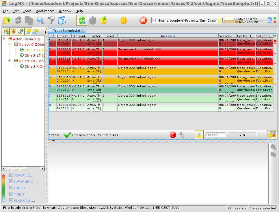
Using the LogMX trace supervisor is surely the most useful way of monitoring the traces, in real-time or post-mortem. As such it is the trace supervisor that is by far the most frequently used.

LogMX offers rich features that allow to:

  • browse conveniently even large sets of traces
  • select the minimum level of detail for the traces to be displayed
  • search traces for specific patterns, or by emitter, date, location, etc.

The only drawbacks of this trace mode are that:

  • it requires a specific (commercial) tool (LogMX), properly obtained, installed and configured with the Sim-Diasca parser
  • the results cannot be directly integrated into a report

LogMX-based traces are the default output type. Should the trace output type have been changed, it can be restored by setting TraceType to log_mx_traces, in traces/src/traces.hrl.

Text Based Traces

Although it is generally less convenient, simulation traces can be inspected directly from any text viewer (hence without LogMX).

If such a reading could be directly performed on the trace file (typically named MY_CASE-by-MY_USER-MY_SII.traces) that is generated by default for LogMX, its formatting is designed for that latter tool rather than for humans, hence is a bit difficult to read in its raw form. A better option is in this case to select a trace format whose outputs are meant to be read directly as they are, as free text.

To do so, in traces/src/traces.hrl, just define TraceType to {text_traces,text_only} instead of log_mx_traces, and rebuild everything above WOOPER (i.e. the Traces package, the Sim-Diasca package, and the code using it).

As a result, simulation traces output in the aforementioned trace file will be in plain text and encoded for human readability (within a nice ASCII-art array); they can thus be then read as are thanks to any text viewer.

By default gedit will be automatically triggered as a trace supervisor, and the user will be requested by the editor to reload that document as newer traces are appended.

If wanting to use another text viewer, just update accordingly the executable_utils:get_default_wide_text_viewer/1 function in the Myriad package (in myriad/src/utils/executable_utils.erl): gedit might be replaced for example by nedit or by xemacs.

Note that only the most interesting trace fields are kept here (a well-chosen subset of the full, actual ones), for the sake of readability.

PDF Trace Report

When wanting to generate a trace report once the simulation is over - rather than monitoring the traces during the simulation, a PDF output can be retained.

To do so, in traces/src/traces.hrl, just define TraceType to {text_traces,pdf} instead of the default log_mx_traces, and rebuild everything above WOOPER (i.e. the Traces package, the Sim-Diasca package, and the code using it).

Then, as soon as the simulation will have stopped, the traces will be properly aggregated and formatted from Sim-Diasca, a PDF being generated and then automatically displayed. This PDF can be useful to share simulation results asynchronously (e.g. with remote colleagues).

Only the most interesting trace fields are kept here (a well-chosen subset of the full, actual ones), for the sake of readability.

Note that this feature implies of course that you have already the proper documentation toolchain installed, which includes the RST converters (python-docutils package) and a PDF viewer (by default, evince will be used).

In the future, we could imagine an enhancement that would allow to convert a trace file generated for LogMX into a PDF, so that the user can generate a report without having to run again the simulation with different trace settings.

However, as simulations are expected to be totally reproducible, it would just a matter of saving some runtime, so the priority of this enhancement is low.

If wanting to use another PDF reader than evince, just update accordingly the executable_utils:get_default_pdf_viewer/0 function in the Myriad package (in myriad/src/utils/executable_utils.erl): evince might be replaced for example by mupdf, otherwise by acroread or xpdf.

Then recompiling this module should be enough.

Probes

The Sim-Diasca probes can collect all kinds of numerical data produced during simulation, and generate a graphical view of them.

Probes are result producers, and as such are dealt with by the result manager.

There are two main kinds of built-in probes:

  • basic probes, the most resource-efficient, scalable ones
  • virtual probes, based on the data-logger, the most flexible and powerful ones

They are based on similar interfaces and share most features, including the management of their rendering.

Among the common features:

  • a probe will be created if and only if it is to produce a result of interest for the simulation, i.e. iff it matches the result specification chosen by the user (in the simulation settings); otherwise this probe will be not created at all, sparing 100% of the resources it would require
  • their data files for time series all start with an header that lists meta-data like generation date and time, probe name, title, and the description of the curves involved

As subclassing the basic probe or devising new ones (e.g. web-based ones) is relatively straightforward, projects may start with built-in probes and define in their course specialised ones.

Another popular option is to switch to dedicated plotting/rendering libraries when post-processing the data resulting from the simulation. Then, in the simulation case of interest, the data_only producer option might be specified in the patterns listed in the result_specification field of the simulation_settings record , in which case only the corresponding data files (*.dat files) will be produced (no *.png plot files).

Generic Probe

A generic probe can be dynamically configured to gather any number of time series, and represent them with as many curves whose abscissa axis corresponds to the simulation time, like in:

Samples may or may not be sent to their probe in chronological order (indeed, depending on their settings, probes may write directly their data to disk, yet timestamping them allows their renderer to reorder them if needed).

An example of the output rendering is:

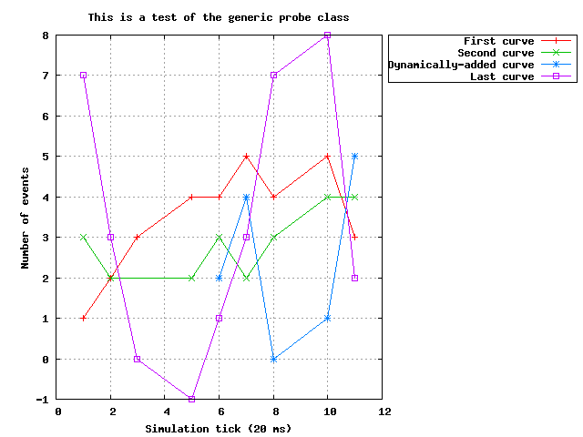
The generic probe is defined in class_Probe.erl, and tested in probe_rendering_test.erl (unit rendering test) and class_Probe_test.erl (integration test).

By default:

  • a probe will create a command file only when requested to generate a report (i.e. not when itself being created, in order to be able to take into account any later change in the curve declarations and rendering options before rendering is requested)
  • the sample data that it will receive will be written to disk on-the-fly (i.e. it will not be cached in memory, in order to minimise the memory footprint of the probes)

Both behaviours can be changed, thanks to construction-time options (see, respectively, the create_command_file_initially and deferred_data_writes options).

As shown in the probe test, new curves can be dynamically declared, so that samples of increasing sizes can be sent over time (in the example, the fourth curve, the purple one, is dynamically added). The corresponding curves will be appropriately rendered the next time a report generation is requested. Existing curves can be renamed as well on-the-fly.

Full time-steps can be skipped, i.e. a new sample might be associated to a tick more than one tick after the previous one, and curve rendering will respect that time lapse (in the example, no sample at all was sent for ticks #4 and #9).

Partial samples can be sent as well, when no data is available for a given curve at a given tick (in the example, the second curve, the green one, had no relevant data for tick #3).

Finally, probes can also support the generation of histograms like this one:

Specialised Probes

Reliability Probes

Once associated with an equipment, a reliability probe, still based on a time series, records at each simulation tick the status of this equipment (functional or in failure), and can generate the chronology of status changes as shown here:

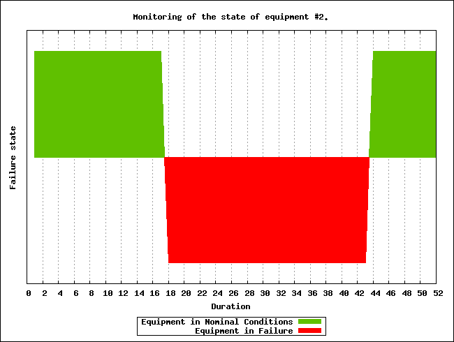
The reliability probe is defined in class_ReliabilityProbe.hrl, and tested in class_ReliabilityProbe.erl.

Probe Troubleshooting

Here are some general troubleshooting hints about probes, when they seem to fail to produce their expected graph renderings.

First, no error nor warning should be output in the terminal or in the simulation traces; otherwise the user code must be fixed accordingly. It can happen for example when no data at all was sent to a probe, whereas it was requested to generate a report.

For each probe that was created, fed with data and requested to be output, a report (a graphical view of its data) should be made available to the user.

By default, a basic probe will perform immediate (non-deferred) writes: otherwise it would have to keep its sample in-memory, potentially exhausting the RAM if the simulation was long enough.

As a consequence, by default, each probe uses one opened file descriptor. This limits by default the maximum number of simultaneously existing basic probes per computing node to roughly one thousand on most systems; having too many of such probes created results in the emfile error being reported - possibly as soon as probe creation, when each of them is to check that its prerequisites are met (typically regarding the gnuplot version available locally).

As this limit is just a shell setting, this can be overcome; for example ulimit -n 20000 will raise the maximum number of open file descriptors from the usual default 1024 to 20000, which is likely to be sufficient for most simulations.

This is nevertheless a transient setting that will be reset at each new shell. This limit is not raised automatically by Sim-Diasca at start-up, as on most systems this would require root privileges - at least, in terms of file descriptor count, above some threshold. For example ulimit -n 2000 may be accepted, whereas ulimit -n 20000 may not, returning then:

ulimit: open files: cannot modify limit: Operation not permitted

A more permanent solution (requiring root privileges) is to use nofile entries in /etc/security/limits.conf. For example one may add following entries to the end of this file (or edit them if already existing):

root soft  nofile 20000
root hard  nofile 40000

As larger numbers of probes are unlikely to generate diagrams that will be actually viewed, just generating and storing the corresponding data samples (no image being then produced) might suffice, in which case the result specifications (as declared in the simulation case) may opt for the data_only producer option (rather than rendering_only or data_and_rendering; refer to class_ResultProducer:producer_option/0).

An even safer option (scalability-wise) is, if relevant, to also tell directly to the probes themselves that no rendering is to be prepared (see the rendering_enabled field of the probe_options record for that).

Probe Report Generation Issues

You must first check that you sent at least one data sample to your probe, and then that it is included in the result specification.

If, when the generation takes place, a warning about bmargin is issued, then you must be using a very old version of gnuplot (e.g. 4.0).

In this case you can either:

  • update your gnuplot version
  • in sim-diasca/src/core/src/probe/class_Probe.erl, disable all key options: set the key_options attribute to an empty string

More generally, if a problems occurs, you should check first that the probe report (e.g. Test_probe.png) was indeed generated.

If yes, it must be a (minor) problem of the display tool, see the ``Probe Report Display Issues``_ section.

If no, actually the PNG could not be generated. The next step is to check in your result directory that the data file (e.g. Test_probe.dat) and the command file (e.g. Test_probe.p) are correct, i.e. existing, not empty, and not corrupted.

If these files seem correct, you can just check that you can generate the lacking PNG by yourself, by issuing on the command line:

gnuplot Test_probe.dat

Depending on the outcome (the PNG is generated, or a gnuplot error is raised), the diagnosis should be easy to determine. Please report to us if a problem remains.

Probe Report Display Issues

Depending on the tool you use for image displaying, multiple graphs may be displayed in the same window: with the default one, Geeqie (geeqie, previously known as gqview), one window may pop up, listing all the graphical results.

If wanting to use another image viewer, you can just edit the myriad/src/executable_utils.erl file, and update accordingly the get_default_image_browser/1 function.

Data-Logger

The purpose of the data-logger is to store and manage simulation data in a more powerful and flexible way than with plain probes.

The data-logger allows any number of virtual probes to be created, and stores them in a distributed database. This allows queries to be done on these data, and outputs to be generated in a very similar way as when using plain probes.

This data service relies a lot on the Mnesia soft-realtime database, which is an Erlang built-in.

One of the objectives of the data-logger is also to allow for an increased scalability: whereas there is a hard limit to the number of co-existing plain probes on any given computing host [31], the underlying distributed tables of the data-logger allow to go one step further, scalability-wise.

[31]Indeed, should probes keep their data in-memory only, their size would grow over simulation time until exhausting the system RAM. Therefore they store by default their data in a probe-specific file instead, but then the maximal number of per-process open file descriptors will kick in, and usually will limit the number of plain probes per simulation node to around one thousand, which may not be sufficient.

Moreover some post-processing across tables can then be done more easily.

The data-logger is defined in the sim-diasca/src/core/src/data-management/data-storage directory.

When running for example the data-logger test (datalogging_test.erl, thanks to make datalogging_run), one can see:

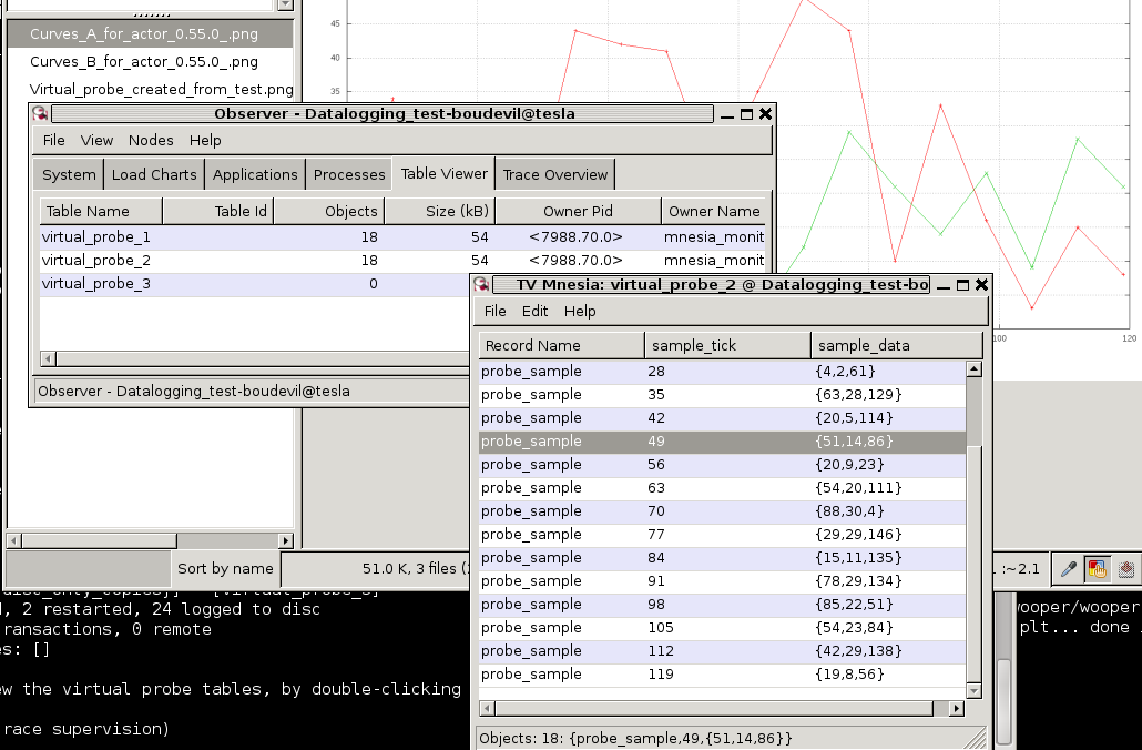
In the stacking of windows, from the upper one to the lower one we can see:

  • a rendering of a virtual probe
  • the list of all known virtual probes
  • the database table corresponding a virtual probe
  • a bit of the console tracking

Console Tracker

The Console Tracker is a lightweight Sim-Diasca built-in which displays live runtime information on a terminal, in order to allow the user to monitor concisely the progress of a running simulation.

A typical output is:

Simulation started at simulation time: 1/1/2000 0:00:00
(tick 3155695199999), real time: 4/12/2010 0:03:31
with a simulation frequency of 50.00 Hz (period of 20 ms).
Simulation will stop no later than tick 3155695260000
(i.e. after 60000 ticks).

Meaning of the console tracker columns:
- S: overall [S]imulation time (full time and date)
- T: overall simulation [T]ick
- R: [R]eal (wall-clock) time
- A: total (distributed) [A]ctor count (load balancer included)
- D: [D]etailed last-tick actor actions
(spontaneous/triggered/twofold counts)
- P: total (distributed) [P]rocess count

Then the tick table [32]:

Simulation Time Tick Offset Real Time Actor Count Detailed Actions Process Count
S: (not started) T: 0 R: 3/12/2010 2:35:54 A: 0 D: 0| 0| 0 P: 64
S: 1/1/2000 0:00:00 T: 0 R: 3/12/2010 2:35:54 A: 900503 D: 0| 0| 0 P: 64
S: 1/1/2000 0:00:00 T: 1 R: 3/12/2010 2:35:55 A: 900503 D: 900503| 0| 0 P: 902626
S: 1/1/2000 0:00:00 T: 3 R: 3/12/2010 2:35:56 A: 900503 D: 900502| 0| 0 P: 902626
S: 1/1/2000 0:00:00 T: 6 R: 3/12/2010 2:35:57 A: 900503 D: 900502| 0| 0 P: 902626
S: 1/1/2000 0:00:00 T: 9 R: 3/12/2010 2:35:58 A: 900503 D: 900502| 0| 0 P: 902626
S: 1/1/2000 0:00:00 T: 12 R: 3/12/2010 2:35:59 A: 900503 D: 900502| 0| 0 P: 902626
S: 1/1/2000 0:20:00 T: 59998 R: 4/12/2010 9:39:00 A: 900503 D: 900502| 0| 0 P: 902626
S: 1/1/2000 0:20:00 T: 59999 R: 4/12/2010 9:39:00 A: 900503 D: 900502| 0| 0 P: 902626
[32]The table has been pretty-printed and considerably shorten.

Finally the simulation summary:

In batch mode, no browsing of results performed. Waiting for their
processing and retrieval.
Results are available now.
Simulation stopped at simulation time: 1/1/2000 0:20:00
(tick 3155695260000), real time: 3/12/2010 9:39:01, after a
duration of 20 minutes in simulation time (60000 ticks),
computed during a wall-clock duration of 7 hours, 3 minutes,
33 seconds and 22 milliseconds.
Simulation ran slower than the clock, with an acceleration factor
of x0.047.

The console tracker is notified of all ticks (and is given the corresponding information), but it selects for display only up to one tick information per second (the latest available), in order not to overwhelm the console and slow-down very fast simulations (thus, each line is a snapshot for a specific tick, not a cumulated value since the last output).

So a simulation run twice will probably display different ticks, thus different information, and this is normal.

One can change the console tracker behaviour so that all ticks are displayed. In this case the tick information from a simulation run twice should match. If it is not the case, there must be a bug, either in Sim-Diasca or in the models.

To switch from one console line per second to all lines being displayed, just edit, in sim-diasca/src/core/src/scheduling/class_TimeManager.erl, the tick_tracker_main_loop/3 function, apply the in-code comments (the ones starting with (uncomment next line), and recompile this module.

Data Exchanger

The Data Exchanger is a distributed simulation service that allows to share conveniently and efficiently data among all actors, even if the data sets are large and the actors numerous.

Objectives

More precisely, the data-exchanger fulfills two technical purposes:

  • to allow for a more efficient, yet safe, sharing of data, based on an automatic distribution that allows all read requests (potentially very numerous) to be performed locally only (i.e. directly on the computing node on which each reading actor is running - thus with very low overhead)
  • to provide a way of propagating data conveniently and as quickly as possible in simulation time, latency-wise: an update made at tick T will be visible to all readers during the full T+1 tick, right from its start, and thus can then be accessed with zero-latency, through any number of direct reading messages per actor (without having to be synchronized thanks to actor messages that would be reordered and executed later); actor-wise, this allows to perform series of any number of (potentially conditional) read requests during the same tick, with potentially arbitrarily complex read patterns, at virtually no performance cost nor developing effort

Each data that is shared according to following conventions:

  • data is defined as key/value pairs, respectively an atom and any Erlang term
  • data can be static, i.e. be defined initially and thus be permanently available (e.g. through the built-in support for reading from configuration files) and/or be introduced in the course of the simulation, i.e. be dynamic
  • can be modified over time once defined (non-const, to be defined with the mutable qualifier) or not (immutable, to be defined with the const qualifier)

Note that static/dynamic and mutable/const are orthogonal properties, all combinations of which making sense.

So, basically, compared to inter-actor messages, the data-exchanger offers an alternate, radically different paradigm to manage data, that can be seen as a DSM (i.e. a Distributed Shared Memory), somewhat a dual approach to the in-tick reordered actor messages. The point is that this service still allows to preserve simulation properties, and that the different trade-offs it offers may, depending on the situation, be more suitable for some needs of information sharings, notably in the one writer/many readers case.

These services had to be offered with care, as, for the model developer, unwanted side-effects or race conditions should not be made easier to perform, and for sure these sharing services must not become a means of bypassing the simulation mechanisms (e.g. if instantaneous reads and writes were allowed, then the induced possible immediate inter-actor communication would break at least reproducibility).

Note that the only standard way of exchanging information and synchronising between actors (as opposed to the sharing of information) remains the sending of actor messages.

Sharing Constant Data

One of the notable use cases of the data exchange service is the sharing of simulation-specific configuration settings: then all actors can have access to the same static (const) data sets, which will be available from the start, before the simulation is started, even before the first initial actor is created. It is then functionally equivalent to having each actor read these information from a common configuration file, except that the reading is done once for all actors on each node, instead of once per actor, avoiding the massive reading and parsing, etc. that would be incurred otherwise.

These configuration files must respect the Erlang term syntax, with a {Key,Value} pair or a {Key,Value,Qualifier} triplet per logical line of the file, ending with a dot. Qualifier is either mutable or const; not specifying a qualifier implies const [33]

[33]And modifying afterwards a (thus mutable) data without specifying a qualifier will make it const then.

Such configuration files are to be declared in the enable_data_exchanger field of the deployment settings (see the detailed syntax in class_DeploymentManager.hrl). They will be then automatically deployed [34] and their corresponding data defined. As a convention, their recommended extension is .cfg (e.g. my_simulation_parameters.cfg). See the valid_example_configuration_file.cfg and invalid_example_configuration_file.cfg as examples.

[34]We preferred adding automatically these user-specified configuration files to the deployment archive and having them parsed once per computing node, rather than read only once and then be sent as messages over the network: for fairly large data-sets, we believe that being compressed in a data archive rather than being expanded as Erlang terms on the sender-side should result in better performances, network-wise.

Of course the data-exchange distributed repository can also be fed at runtime, as opposed to statically (i.e. through configuration files). And this can be done initially (before the simulation is started), through method calls (see the define_initial_data/{1,2,3,4} static methods to define new data entries, and the modify_initial_data/{1,2,3,4} static methods to update them once defined) or from an actor (see the class_Actor:define_data/{2,3,4} and class_Actor:modify_data/{2,3,4} counterparts helper functions), thus either initially as well, or in the course of the simulation.

For an actor to be able to use the data-exchange service, it must first update its state with the class_Actor:enable_data_exchange/1 helper function. See class_DataExchangeTestActor.erl for a complete example. Note then that its subsequent reads (and commits) may happen whether the simulation is already running or not (the latter case applies to initial actors).

So, during any given tick, each actor can freely perform from the data exchanger immediate, direct (zero-latency, as not based on an actor message) read operations of any number of data-sets, and the developer can be confident that this will be done in the most convenient, safe and reliable, performance-efficient, scalable way.

Reciprocally, instead of being read, new data can be defined, or existing data can be modified, provided of course it was declared as non-const (i.e. with the mutable qualifier), as discussed in the next section.

Modifying Data

Any already-defined data, whose current qualifier is mutable, can be modified, either initially (in this case the change will be immediate) or in the course of the simulation (in this case the change will occur only starting from the next tick).

This is done thanks to calls to the modify_data/{3,4,5} helper functions, which on each tick are synchronous operations resulting in the root data exchanger recording all commits that happen during the current tick, and checking them on the fly (e.g. no change in const data, only up to one commit per data key per tick, etc.). A commit request is implemented as a direct message sending, from an actor to the root data exchanger (thus not going through the data-exchange tree).

Once this tick is over, should at least one commit have been requested, the root time manager notifies the root data exchanger that we are in-between two ticks and that it can thus propagate safely its commit(s), down the exchanger hierarchy (tree-based propagation).

Once done (i.e. fully acknowledged by a reverse, leaves-to-root, traversal), the root exchanger notifies the root time manager that the next scheduled tick can be triggered.

That way, at the expense of a minimal (and conditional [35]) inter-tick wall-clock latency [36], all subsequent readings then done can be performed locally (on an exact local clone of the root exchanger) and instantly (with a zero-tick latency in virtual time): indeed, during a tick, from the point of view of actors, no data can change; their update will happen only in-between ticks, so all reads can be done

[35]If no commit is done during a tick, the data-exchanger will incur virtually no overhead, so this data-exchange service will cost resources only if used.
[36]For synchronisation reasons, the commit propagation has to be part of the critical path of the time manager (the period between two ticks during which no parallel operation can occur). As increasing too much that duration would directly impact the simulation overall performances, we did our best to minimise the inter-tick latency induced by the data-exchange service. For example most checkings are not once a write operation is requested, not later once it is to be actually committed.

Note also that setting a data involves either defining a new key or modifying a value associated to an already-defined key, possibly also updating the qualifier of a key/value pair, provided these operations are licit (e.g. a mutable qualifier may be set to const, not the other way round; a data can be defined only once, and modified any number of times once first defined).

More precisely, data modification, during the simulation, is to be done from actors, and is either:

  • defining new data, with class_Actor:define_data/{2,3,4}
  • or modifying pre-existing data, with class_Actor:modify_data/{2,3,4}

The point is that, once the simulation is started:

  • a modification done at tick T will be visible (thanks to read operations) only at the next scheduled tick (e.g. T+1)
  • a given data (i.e. a value associated to a key), provided it was declared as mutable, can be modified during the simulation up to once per tick, otherwise the data exchanger will detect the mismatch (commit inconsistency, up to one writer per key and per tick) and crash on purpose the simulation with a relevant exception

So if the data exchanger holds at tick T a {my_data,AnyTerm} mutable entry, and if during this tick an actor commits a {my_data,AnotherTerm} entry, then during T all read requests of my_data will return AnyTerm, and during T+1 they will all return AnotherTerm. If more than one actor attempts to commit at T a change to my_data, then the simulation will fail. Even if they try to commit the exactly the same value.

Practical Use

The data-exchange service is activated by default, as its runtime overhead in case it is not actually used is fairly low.

It can be explicitly enabled or disabled through the deployment settings, see the enable_data_exchanger field of the deployment_settings record, defined in class_DeploymentManager.hrl. It is also the place where the list of configuration files to be used for static information (if any) can be specified.

Data can be defined, then modified and/or read.

When a data is to be read, only its key is to be specified.

When a data entry (key and at least value) is specified either for definition or for modification, if no qualifier is specified, then the default one (const) will be implied. This means that requesting a modification with a data entry {my_data,AnyTerm}`` implies notably that:

  • my_data has already been defined
  • its previous qualifier was mutable (thus was explicitly set as such), otherwise the modification would be bound to fail
  • its new qualifier will be const (none was specified in the modification request), thus no further modification will be done on that data

These data operations can be made either from the simulation case (thus, before the simulation is started) and/or from actors (before or during the simulation).

Implementation Details

There is one data exchanger agent per computing node, and they form a tree (the exchanger hierarchy), whose root is the root data-exchanger, very much like the one of time managers.

That way commit consistency is verified by the root data exchanger, which holds the sole reference copy of the data repository, which is replicated on all non-root (i.e. local) data exchangers. As updates are made between ticks, during a tick the data is stable, and each actor will be able to read them locally, and at will.

Data definitions and modifications will be recorded during a tick, and applied once that tick is over, before the next scheduled one.

Data can also be defined and modified before the simulation is started. Definitions can be done through requests or through the reading of any number of configuration files.

For actors, data readings are just plain, direct, non-reordered, WOOPER requests that are made locally (on the node of the reading actor), thanks to the local exchanger that was automatically deployed there. Therefore readings should be considered as being by design fast and inexpensive.

From the simulation case, the readings are managed a bit differently internally, depending on whether the user host is included or not in the simulation.

If included, then on that same user host there is a computing node with its own local data-exchanger. As a consequence, to avoid a data duplication of the exchange repository on the user host, the user node will interact with the data-exchanger local to the computing node on the same host.

If the user node is not included in the simulation, then there is not computing host to rely upon, and a local data-exchanger dedicated to the user node is simply created and integrated in the data-exchange hierarchy.

Spatialised Support

Overview

Currently only a support for 2D environments is provided - of course the user might define any number of other environments if wanted.

The spatial environment is embodied by an instance (a singleton) of class_TwoDimensionalEnvironment.

The support for low-level spatial computations is provided by the linear_2D module (in myriad/src/maths).

Distances are expressed in meters, speeds in meters per second.

The simulated world has an origin ({0.0,0.0}) and spreads in both dimensions. Cartesian coordinates are used.

By default the world is a torus, i.e. the coordinates wrap around. They range from the origin to {XMax,YMax}.

Spatialised Elements

A simulation element that is spatialized has a position in the simulation world, and should be (directly or not) an instance of class_SpatializedEntity or, more precisely here, a class_TwoDimensionalSpatializedActor.

The constructors of each of these classes take, as first actual parameter, the PID of the environment. An upper bound of the speed of each instance may be specified (it allows to optimise the mode of operation of the environment).

This class_TwoDimensionalSpatializedActor class defines an attribute position whose type is linear_2D:point() and a -spec getPosition(wooper_state(),pid()) actor oneway which triggers back on the caller, at the next diasca, the -spec notifyPosition(wooper_state(),linear_2D:point(),pid()) actor oneway.

Interaction with the Environment

In the general case, no instance is able to know the whole simulation world. An instance is only able to perceive a subset of it, through its perception.

Such a neighborhood can only be obtained thanks to a specific actor, the environment.

An instance can indeed call the actor oneway defined, here in class_TwoDimensionalEnvironment, as -spec getEntitiesWithin(point(),radius(),pid()): it requests that the entities within a disc whose center and radius are specified are determined by the environment.

This center of perception must be by convention the current location of the perceiving instance, as:

  • a given instance should only perceive its own neighborhood
  • the environment will take advantage of this call to update its knowledge of the location of the perceiver

Sim-Diasca Helper Tools

These tools are not strictly necessary to the mode of operation of the engine, however they provide some features that are very useful in some contexts.

As a consequence, on a vanilla Sim-Diasca version, they start disabled (so that they induce no resource overhead), but their sources are in the main codebase, they are always built and readily available - as soon as the user chooses to activate them.

Performance Tracker

The Performance Tracker is a fully optional mechanism that allows the user to monitor a simulation that was run, in order to profile it.

It aims to monitor and then generate reports giving detailed information about all kinds of technical measurements dealing with performances, notably in terms of resource consumption (CPU, RAM, network, Erlang process count, etc.).

Requirements & Functional Coverage

The current version provides the following features:

  • trace the following memory consumptions on the user node and on computing nodes along with the simulation duration or with the wall-clock time:
    • the available memory (which is: free memory + buffers + cache)
    • the memory used by the other applications (i.e. all non-Erlang applications)
    • the memory allocated to the Erlang emulator (i.e. the memory currently used by the simulator), plus any other Erlang program being executed at the same time
    • the used swap
  • trace the overall number of Erlang processes (on a per-node basis) during the simulation in real (wall-clock) time and/or in simulation time (tick)

In the future, it will allow to trace also:

  • overall number of instances of a given class; for example: how many classical or virtual probes, or class_Foobar instances on each node
  • the wall-clock duration of each simulation tick, on each node

The output of the performance tracker is:

  • time series (.dat files)
  • and/or the corresponding graphs (.png)

Its reports are available post-mortem (not live), among the simulation results.

Implementation

The performance tracker and its integration test are located in sim-diasca/src/core/src/data-management/monitoring/performance.

The performance tracker is integrated at the Sim-Diasca level (i.e. not only at the WOOPER-level), and relies on various services of the engine (e.g. probe, deployment manager, result manager).

The performance tracker is implemented as an optional service, disabled by default (to avoid any unnecessary runtime overhead), which can be enabled on a per-need basis.

It defines following classical probes:

  • a global probe is created in order to track the overall number of Erlang processes on each node: it includes as many curves as there are nodes (user node and computing nodes); each curve is named according to its corresponding node
  • a probe per node is also created in order to track the resource consumptions on each node

In terms of architecture, currently the performance tracker is centralized (a singleton) and is created on the same node with the Depployment Manager in order to enable the performance information available in all circumstances, such as, simulation fail because of a timeout or a computing node crash.

In case of performance tracker enabled, the data for the probes is retrieved in a predefined interval during simulation, by default, this interval is defined as 100ms and it can be modified by sending a "setTickerPeriod" message with new interval to the performance tracker.

In the future and in particular for the scalability test when numerous computing nodes are engaged, there will be a performance monitor per node besides this centralized tracker, in order to reduce the exchanges over the network. Contrariwise, the distributed monitoring way can lead to lose some node performance information when a node is crashed during the simulation and relevant data saved on it.

Performance Tracker Activation and Creation

The activation of the performance tracker is to be requested from the simulation case, through its deployment settings: the enable_performance_tracker field of the DeploymentSettings record (defined in class_DeploymentManager.hrl) must be set to true.

When the performance tracker is enabled, the user can customise it according to her needs, notably in order to set the wall-clock period, expressed in milliseconds, between two measures (performance tracker samples); see its setTickerPeriod/2 method.

To do so, the PID of the tracker must be obtained, thanks to the following static method:

MyPerformanceTrackerPid = class_PerformanceTracker:get_tracker()

Performance Tracker Report Example

Example 1: a single-host simulation

These reports are generated based on the results of the performance tracker test (class_Performance_Tracker_test.erl) with following test configuration:

  • only one initial test actor (class_PerformanceTracker_TestActor)
  • each test actor creates a new test actor every 4 simulation tick
  • the total simulation duration is 36 simulation ticks
  • the simulation runs on only one machine, that means: the user node and the computing node are on the same machine

One can have a global view of the simulation, first in wall-clock time:

The same global view can also be shown in simulation time:

More detailed information can be collected, on a per node basis. Here first is the report specific to the user node, in wall-clock time, then the same report for a computing node:

Example 2: a simulation distributed over 4 nodes

These reports are generated based on the results of the performance tracker test (class_Performance_Tracker_test.erl) with following test configuration:

  • only one initial test actor (class_PerformanceTracker_TestActor)
  • each test actor creates a new test actor every 4 simulation tick
  • the total simulation duration is 36 simulation ticks
  • the simulation runs on 4 machines, that means: the user node and one computing node are on one machine, the three other computing nodes are on three different machines

One can have a global view of the simulation, first in wall-clock time:

The same global view can also be shown in simulation time:

More detailed memory consumption information can be collected. Here first is the report specific to the user node, in wall-clock time, then the same report for computing nodes:

Post-Processing Services

As hinted by their name, these services are not integrated to the engine, but are to be applied, if needed, to the results it produces.

Time-Series Analyzer

Time-series are typically produced by simulation probes (either basic or virtual), and are stored in *.dat files, which gathers the values of a series of curves at different ticks.

Such files can be inputs to the Sim-Diasca analyzer tool for time series, which can then apply them various algorithms, some related to signal processings.

For a time-series file, identified processings of interest are:

  • select a subset of curves in a time-series file
  • remove empty ones and/or constant ones
  • generate a basic gnuplot command file corresponding to a .dat file

For a curve, identified processings of interest are:

  • find the extrema (minimum and maximum values), and when they occur (list of matching ticks)
  • compute the average value of the curve (which is not necessarily the average of the values, due to potentially non-consecutive ticks)
  • apply a convolution filter on the curve samples
  • compute the curve for the moving average (a specific case of convolution), which is a way of obtaining a smoother curve, making its interpretation easier by highlighting trends
  • perform a linear interpolation between samples
  • perform decimation, to reduce the number of samples
  • change scale (e.g. switch to logarithmic, reshape to fit into a 0..1 interval, etc.)

Plugin Infrastructure

Sim-Diasca offers a full Plugin Management System, which allows third-party code to interface with the engine in various ways.

General Principles

Each plugin is able to:

  • specify requests for configuration changes (e.g. like the number of sequencers on each computing node)
  • know runtime information, like the list of the computing nodes that have been actually elected by the engine
  • be notified of all main events (engine-related or even case-defined) regarding the simulation, which for example allows tools to monitor resources during only some phases of the simulation - typically when models are effectively evaluated (skipping deployment, preparation, initialisation phases, as well as the ones after the simulation)

More In-Depth Description

A simulation case can specify a list of directories that will be scanned for plugins at start-up by the engine.

This is done thanks to the plugin_directories field of the deployment_settings record, which can be set to a list of directory paths (either absolute or relative to the directory where the case was launched). See city_benchmarking_test.erl (in mock-simulators/city-example/src) for such an example case.

Each BEAM file found in any of these directories is expected to comply with the interface described in the sim_diasca_plugin behaviour [37] ).

[37]This is a post-R15B, Dialyzer-friendly, behaviour. It is defined in sim-diasca/src/core/src/plugins/sim_diasca_plugin.erl.

This boils down to implementing a callback for all simulation events:

  • on_simulator_start: when the simulator is started (or almost, as basic services, including the trace one, are already up)
  • on_deployment_start: when the deployment phase starts
  • on_deployment_stop: when the deployment phase stops
  • on_technical_settings_available: when the simulation technical settings are available, notably once the deployment phase is over
  • on_case_initialisation_start: when the simulation case starts the creation of the initial state of the simulation
  • on_case_initialisation_stop: when the simulation case finished the creation of the initial state of the simulation
  • on_simulation_start: when the simulation is started (first tick, first diasca)
  • on_simulation_bootstrap_start: when the simulation is just started and must evaluate the first diasca of all initial actors
  • on_simulation_bootstrap_stop: when the evaluation of the first diasca of all initial actors is over
  • on_simulation_wallclock_milestone_met: when a wallclock milestone is met (i.e. when a given duration in real time elapsed)
  • on_simulation_tick_milestone_met: when a tick milestone is met (i.e. when a given number of ticks have been evaluated)
  • on_simulation_stop: when the simulation is stopped (an ending criterion was just met; only called on successful ending)
  • on_result_gathering_start: when the results start being gathered, after simulation termination
  • on_result_gathering_stop: when the results have been gathered
  • on_simulator_stop: when the simulator execution stopped under normal circumstances (i.e. not crashing)
  • on_case_specific_event: triggered iff a case decided to notify the plugins of a specific event

Most callbacks just take one parameters, the current plugin state, and return one value, the new plugin state.

This allows stateful plugins to be easily implemented (instead of, for example, spawning a dedicated and registering it), the engine keeping track of their state between callbacks. Of course using that feature is optional and, for example, all callbacks can ignore the engine-specified state and only return the undefined atom as new state.

Some callbacks are a little more complex:

  • on_simulator_start/2 is given also the current configuration changes (as possibly already updated by other plugins - the first of them receiving a blank configuration_changes record), so that the currently executed plugin can update it
  • on_technical_settings_available/2 is given also a technical_settings/2 record, describing the actual settings then enforced by the engine, notably on the basis of the previously consolidated plugin configuration requests
  • on_simulation_wallclock_milestone_met/2 and on_simulation_tick_milestone_met are respectively also given the current simulation timestamp (respectively in real and virtual time), whenever a milestone is met
  • on_case_specific_event/3 is given the name of the corresponding case-specific event (as an atom) and its associated data; see class_CityGenerator.erl for an example of use

Implementation Notes

All services of the lower layers are available to plugins. As a result, they can rely upon the facilities of the Myriad layer, WOOPER classes may be used as plugins, and the distributed trace system can be used by the plugins as well.

The plugin service is mostly located in sim-diasca/src/core/src/plugins.

An example of a full, complete plugin is available in plugins/tests/my_plugin_example.erl.

We might consider supporting even distributed plugins (with one instance of them, code and data, being deployed and run on each computing node), if such use case was found interesting.

Sim-Diasca Modelling Guide

Objective & Context

The goal here is to help bridging the gap between the modelling world and the simulation world: in this section we discuss what is the "language" that the simulation engine natively understands, so that a modelling team is able to prepare descriptions of models that can be almost readily implemented into actual (runnable) simulation models.

Basics Of Simulation Operation Mode

Actors & Models

Actor

A simulation actor is the basic building block of a simulation. It is an autonomous agent, usually corresponding to an element of the simulated system, which, during the course of the simulation, will be automatically and appropriately scheduled.

Being scheduled means being given the opportunity to act, either spontaneously and/or after having been triggered by another actor.

Each actor has a private state, which is made of a set of any number of attributes.

An attribute has a name and a value, which can be of any data type, usually made of an arbitrarily-complex combination of primitive types (integer, logical text constant [38], floating-point value, etc.) and structures (fixed-size array [39], list, tree, associative table, etc.).

[38]Named atom in Erlang.
[39]Named tuple in most declarative languages, including Erlang.

For an actor, acting corresponds mostly to:

  • changing its private state (e.g. changing the value of an attribute)
  • sending messages to other actors (e.g. to notify them that some event occurred)
  • possibly, triggering side-effects (e.g. sending a message to the distributed trace system)

Note

Please refer to the Sim-Diasca Developer Guide for more implementation-level information about actors.

Model

A model corresponds to the description of a type of simulation actors, regarding state and behaviour.

Technically a model is actually a specific class, whose instances are the simulation actors that respect that model.

Expressivity

Of course, Turing machines can be simulated, but more generally very few restrictions apply to models, which can be arbitrarily complex.

The most difficult issue to deal with comes probably from the latency (in virtual time) which is induced by the simulation mechanisms: an information (i.e. an actor message) sent at tick T cannot be processed by its recipient sooner than tick T+1.

This one-tick latency can be alleviated by increasing the simulation frequency. It will then just be a matter of choosing the preferred trade-off between latency and wall-clock simulation duration.

Time-Stepped Simulation

Models and actors have to comply with the operating conventions of the Sim-Diasca simulations.

In that context, the main convention is that these simulations are time-stepped. This means that the simulation time is sliced into chunks of constant durations.

Therefore we can define at which frequency a simulation should run: a simulation scheduled at 50Hz will rely on a fundamental period of 1/50 = 20 ms, thus all simulation time-steps (also known as ticks) will correspond to 20 ms of virtual time.

Uncoupling From Virtual Time

Actors are only aware of the passing of this simulation virtual time: the actual time that we, users, experience must not matter to them, otherwise the simulation would loose most of its expected properties.

For example, we do not want the same simulation to output different results depending on the processing power that happens to be available for it.

Thus, for an actor, whether the computing of a given virtual 20ms time-step actually lasts for 1 ms or for two minutes of our time shall be irrelevant; each of these 20 ms time-steps will last in our time exactly as long as needed to compute it appropriately, and the processing of two successive time-steps might require vastly different actual durations, in user time.

Formalisation

Modelling allows to bridge the gap between our knowledge of the system and its implementation in the context of a simulation. Generally, increasingly detailed models are specified: first as full text, then with more formal languages.

One can certainly use flowcharts:

But one may preferably rely on a few UML diagrams, including:

  • use case diagram
  • activity diagram
  • class diagram
  • sequence diagram

Other interesting diagrams might be:

  • communication diagram
  • state machine diagram

This is one of the most delicate steps, as often the domain experts are not able to write by their own their corresponding models: they generally make use of domain-specific languages, which are tailored for their needs but quite often are, simulation-wise, not standard.

So a translation step to the simulation language must generally take place, and usually domain experts cannot perform that work [40].

The best practice we recommend is to adopt a unified language to specify all models first, and to practise pair-work (one domain expert sitting on the side of a computer scientist/model developer) to ensure that the translation is correct. Indeed, mistakes can easily be made:

[40]These restrictions surely apply to, say, lower-level C++-based simulation engines which demand that models are written that way; and, more generally, models whose behaviour is intrinsically to be described algorithmically need anyway a programming language to be specified. However some of these languages are more suitable than others. To take a real-life example, for the CLEVER project, 5 days of Erlang training, 5 days of basic Sim-Diasca training and 3 days of advanced Sim-Diasca training have been sufficient so that a team with no prior knowledge about these topics was able to write not only models but even a whole specialisation layer of Sim-Diasca for the simulation of metering systems.

Actor Messages

Actors can communicate only thanks to the passing of specific messages, named actor messages.

During one tick, any actor can send any number of actor messages to any number of actors.

When an actor A sends during tick N an actor message to actor B, B will process it only during the next tick, N+1 [41].

[41]This 1-tick latency is induced by the time-stepped nature of the simulation. This is a constraint indeed, but it can be alleviated (for example by anticipating exchanges and/or choosing a higher fundamental frequency for the simulation) and it is at the root of all the useful properties these simulations can rely on.

A corollary is then that if A requests an information from B during tick N, A will process that information during tick N+2.

Moreover during a tick an actor may receive multiple messages from multiple actors. No assumption should be made on their processing order within that tick, as the simulation algorithm will have reordered them to ensure the respect of the simulation properties (e.g. reproducibility or ergodicity).

Actor Life-Cycle

Actor Creation

An actor must be either created:

  • by the simulation scenario, before the simulation is started
  • by another (already synchronised) actor

In the latter case, if actor A requires the creation of an actor B during tick T diasca D (hence at {T,D}), then B will be actually created at tick {T,D+1}. On the next diasca ({T,D+2}) B will be scheduled for the first time (thanks to a call to its onFirstDiasca/2 actor oneway), while A will be notified of this creation (and of the PID of B).

Usually some specific actors, not directly corresponding to an element of the target system, are defined to create other actors.

For example a deployment policy for an information system can be such an actor, that will create devices according to a given statistical law, in the course of the simulation.

The simulation scenario itself can be modelled as one of these creating actors.

The actual creation of an actor in the course of the simulation is made of a few steps:

  • at {T,D} the creating actor issues a creation request [42] to the load balancer
  • at {T,D+1}:
    • the load balancer processes that request, and creates synchronously the corresponding instance on the computing node it deems the most appropriate
    • during its construction the instance retrieves the overall scheduling settings from the time management agent it is in contact with, and as a consequence notifies it of how it intends to be scheduled; as the created actor is not synchronised yet to the simulation, its initial construction stage has to respect some restrictions; notably the actor is not able yet to interact with other actors or to consume stochastic variables yet
    • the load balancer sends back to the creating actor an actor message carrying the PID of the created instance, whose basic construction is finished (its constructor ended), but which is not ready to enter the simulation yet
  • at {T,D+2}:
    • the creating actor processes the notification of the created instance, which includes its PID
    • the created actor is notified that the simulation has started for it (it is necessary as it could have been created before the simulation was started) and is scheduled for the first time; it is up to its model to determine whether this actor is ready to develop its behaviour immediately, as it may not have achieved its full initialisation yet (e.g. it may be waiting for other actors to be themselves ready, and/or it might need to set some stochastic values to complete its initialisation, etc.)
    • as soon as the created actor deems it is itself ready (maybe from its first scheduled tick, maybe on later ticks), automatically any related actions will be triggered, and any actors waiting for that actor will be notified that it is ready now; then on the next tick the actor will be free to develop its normal behaviour; by default during its first scheduled tick an actor will not wait for any other actor, and therefore will call directly its (possibly overridden) onReady method; it will then be ready to develop its actual behaviour only on next tick (N+3)
[42]To preserve the simulation properties, the load balancer is itself a simulation actor and therefore the creation request is an actor message.

Actor Deletion

An actor can decide to be removed from the simulation, usually before being deleted.

The removal process from the time manager will then be automatically conducted, but it is the responsibility of the the removed actor to ensure that no other actor will try to interact with it any more.

Usually the underlying logic ensures that it will be so, or the actor to remove notifies relevant actors of its ongoing removal.

Scheduling Sequence

At each fundamental simulation tick, each actor may or may not be triggered by the time manager.

If an actor message was sent to it during the last tick, then the actor will automatically process that message, regardless of its scheduling policy.

Then, the time manager determines whether the scheduling policy of this actor implies that it should develop its spontaneous behaviour during this tick.

If yes, the actor will be notified of the current tick and be requested to act according to its planned behaviour.

If no, the actor will not be specifically contacted?

Stochastic Variables

An actor may rely on any number of stochastic variables, each of which following any probability density function.

Sim-Diasca provides three of the most usual stochastic laws: uniform, Gaussian and exponential. User-specified laws can be added quite easily.

Once synchronised, an actor can draw any number of stochastic variables for any law during one tick, immediately (i.e. with a zero-tick latency).

Main Choices In Terms Of Actor Modelling

Fundamental Frequency

As discussed previously, the root time manager in charge of a simulation will maintain its virtual time based on the fundamental overall frequency the simulation user specified: this frequency (e.g. 50 Hz) directly dictates the duration in virtual time between two successive engine ticks (e.g. 20 ms).

Therefore once this root time manager will have determined that all the actors to be scheduled this tick (the ones having to process actor message(s) and/or having to develop their behaviour on that tick) have reported that they have finished taking that current tick into account, it will then just increment the simulation tick, since the corresponding virtual 20 ms will have elapsed, and then declare that a new tick just has just begun.

Relying on a fundamental simulation frequency does not imply however that each and every simulation actor will have to be scheduled according to that exact overall frequency, i.e. at each tick. Each model is able to pick a scheduling policy that match best its needs.

Once all models have been established, the overall frequency of the simulation can be determined: it should be chosen at least equal to the highest frequency of the models involved.

Policies in Terms of Actor Scheduling

Generally the fundamental frequency will have been chosen so that the most reactive actors can be scheduled at the exact pace they require, but usually there will be also many other actors whose behaviour does not need to be evaluated as frequently.

Therefore, to ease the implementation of models and to preserve performances, the Sim-Diasca simulation engine allows models to request a scheduling more flexible than "every actor is triggered at each simulation tick".

Scheduling-wise, the three most common types of actors are:

  • periodical actors: an actor requesting a scheduling period of N would be triggered by the time manager one time step every N elapsed; therefore an actor could run, in virtual time, at a frequency of 10 Hz even if the fundamental frequency of the simulation was set for example to 50Hz
  • step-by-step actors: when such actors finish a time step, they may specify the next tick at which they should be triggered again (look-ahead), unless they receive an actor message in-between, in which case they may withdraw their already planned activation and set a new one, earlier or later
  • purely passive actors: these actors have no spontaneous behaviour, they are triggered only when they receive a message from another actor during the previous tick

These scheduling policies - and many others - can be implemented with Sim-Diasca thanks to the definition of future actions: each actor, during its triggered and spontaneous behaviours, is able to specify, if needed, a future tick at which it should be scheduled for a spontaneous behaviour.

Thus periodical actors will just define at the end of their spontaneous behaviour one future action which is to take place a fixed duration (in simulation time) after the current tick, step-by-step actors will define arbitrary future actions, and passive actors will never define any specific future action.

Frequency-Independent Timings

In the context of a model, durations (in virtual time) are encouraged to be defined explicitly, absolutely, rather than directly as a given number of simulation ticks, so that models remain as much as possible independent from the actual frequency a simulation is running at.

For example, when a simulated device starts a new task and thus has to determine when a priori it will have finished the corresponding work and be available again, its model may evaluate the corresponding duration to "1400 ms" (in virtual time) rather than directly to an hard-coded "28 fundamental ticks".

Then only (i.e. at run-time), that duration, depending on the actual settings of the current simulation, will be converted to the appropriate number of ticks, so that a change in the simulation fundamental frequency will not impact models.

Note

Using such absolute durations is not always straightforward, as being based on a fundamental frequency leads to a quantisation of durations: if for example a simulated device is scheduled by the voltage of the main supply (say, 50Hz), and if the simulation does not run at a multiple of 50Hz, then either the model will have to ignore the errors resulting from the approximated scheduling, or be designed - if possible - to accommodate to an arbitrary scheduling frequency, in spite of the issues this implies (like the accumulation of rounding or sampling errors).

Modelling Process

Here are the questions that should be addressed simulation-wise, when writing a model.

Nature Of The Model

Should all concepts to be ultimately simulated be represented by models of their own? Sometimes using a simple data structure owned by another actor is the most appropriate approach.

If a concept:

  • is used in multiple different contexts
  • and/or is used by multiple actors
  • and/or has a complex state and/or behaviour
  • and/or is not tightly coupled to any model

then most probably this concept should be mapped to a specific model, i.e. a dedicated class inheriting from class_Actor.

Model Temporality And Reactivity

Supposing we determined that the model was to be implemented as a class, we must then establish whether this model is able to perform spontaneous actions.

If yes (i.e. its instances are able to trigger actions not directly related to the receiving of a message received from other actors), then this is an active actor that will have a spontaneous behaviour, possibly periodical or erratic (step-by-step), etc.

The model is then able to specify with a total freedom its spontaneous scheduling, using notably addSpontaneousTick/2, addSpontaneousTicks/2, withdrawnSpontaneousTick/2 and withdrawnSpontaneousTicks/2, from its actSpontaneous/1 oneway or any of ithe actor oneways it defined.

Please refer to the Sim-Diasca Developer Guide for further details.

State And Behaviour Of The Model

These are very model-specific, but general rules still apply.

Processing an actor message and acting spontaneously both boil down to writing an appropriate method, which may send actor messages and/or return any updated state and/or trigger the removal of that actor.

Triggered Behaviour: Receiving of an Actor Message

For example if an actor A needs to set the color of an actor B, then it may send to it an actor message specifying {setColor,red}. Then, B will process it at the next diasca: its setColor method (actor oneway) will be automatically called and, based on the transmitted parameter, B will be able to update its state, for example by setting its color attribute to red.

Should B receive an actor message requesting an answer (e.g. getColor), it would do so by sending back another actor message to A, like {notifyColor,red}.

Spontaneous Behaviour

It is simply implemented by the calling of the actSpontaneous oneway method of that actor.

See also the Sim-Diasca Modeller Guide for a more in-depth discussion about modelling and implementation, based on a light yet complete example.

Validating The Resulting Simulators

Adding to Sim-Diasca (the simulation engine) a set of models and at least one simulation case results into building a new simulator.

This simulator may or may not be accurate, and this must be established first.

Indeed, drawing bad conclusions from false assumptions or improper reasoning is surprisingly easy:

Being able to trust this new simulator is of course of the utmost importance.

Therefore, before using it to learn new facts, one must validate it adequately.

Validation can be done thanks to multiple non-exclusive approaches, mostly based on the produced results:

Sim-Diasca Cheat Sheet

Warning

This section would deserve some update.

Note: unless specified otherwise, mentioned tests are to be found in the sim-diasca/src/core/src/scheduling/tests directory.

Which Sim-Diasca Version Should Be Used?

Previously there were two versions, one local, one distributed. Now that they have been merged into a single base, one should simply pick the latest stable version. That's it!

To check which version you are using, simply run from the root directory:

$ make info-version
This is Sim-Diasca version x.y.z.

Alternatively, look at the SIM_DIASCA_VERSION variable in sim-diasca/GNUmakevars.inc.

As upgrading the Sim-Diasca version is fairly straightforward, we recommend to stick to the latest stable one, which simplifies considerably any support.

Finally, the lower layers (namely Erlang itself, Myriad, WOOPER and Traces) have of course their own version as well, and the same holds for the upper layers, i.e. the actual simulations making use of Sim-Diasca (from the toy examples in mock-simulators to any user-provided one).

Anyway, as a given version of Sim-Diasca is delivered with all its strictly mandatory prerequisites except Erlang, no particular checking of their version is necessary, as they collectively form a consistent bundle.

How Can We Run a Simulation?

A simulation can be run either from a test file, whose name is suffixed with _test.erl (e.g. stored in a my_foobar_test.erl) or from a case file, whose name is suffixed with _case.erl (e.g. stored in a my_baz_case.erl).

No runtime difference is made between these two (they are technically exactly handled the same), the purpose of this distinction being solely to help the user separating the more punctual testing from full-blown simulation cases.

So, with both tests and cases:

  • the corresponding simulation shall be run by executing a make target bearing the same name, suffixed by _run; respectively as make my_foobar_run and make my_baz_run for the two examples above
  • all files and directories generated by the simulation (notably traces and results) will be created in the current directory; typically the user changes to the directory where the corresponding test or case file is stored, and run it from there
  • by default, simulations will be run in interactively, i.e. with graphical windows popping up (e.g. to browse traces, results, etc.); to prevent that and remain in a purely textual, command-line, batch execution, one can add the CMD_LINE_OPT="--batch" option to the make command; as it involves some typing, it may be convenient to define a shorthand for that, typically by putting in ones's ~/.bashrc a line like: export BATCH='CMD_LINE_OPT="--batch"'

As a full, concrete example of running a test simulation interactively:

$ cd mock-simulators/soda-test/src
$ ls soda_stochastic_integration_test.erl
soda_stochastic_integration_test.erl
$ make soda_stochastic_integration_run
Running unitary test soda_stochastic_integration_run (third form) from soda_stochastic_integration_test
[...]
End of test soda_stochastic_integration_test
(test finished, interpreter halted)

To run a simulation case, here in batch mode:

$ cd mock-simulators/soda-test/src
$ ls soda_platform_integration_case.erl
soda_platform_integration_case.erl
$ make soda_platform_integration_run CMD_LINE_OPT="--batch"
Running simulation case soda_platform_integration_case
[...]
End of case soda_platform_integration_case
(case finished, interpreter halted)

Of course, with the aforementioned shell shorthand, the last case could also be run as:

$ make soda_platform_integration_run $BATCH

How Can I Select Whether A Simulation Run Shall be Purely Local, or Distributed?

Each simulation case is able to define how it is to be deployed or executed, simply by setting accordingly the computing_hosts field in its deployment_settings record (whose full definition and associated comments can be found in class_DeploymentManager.hrl).

Most test cases rely on default settings, which operate this way:

  1. if a host file - named by default sim-diasca-host-candidates.txt - is found in the current directory (the one from which a test case X is run, thanks to a make X_run for example), then the engine will read it and try to use the hosts listed there; the (ETF) syntax is simple and described in the sim-diasca-host-candidates-sample.txt example file, to be found in the sim-diasca/conf directory (it is also described here)
  2. if this host file is not found, the simulation will run only locally

The computing_hosts field can also directly list the hosts involved, but we do not recommend doing so, as in general a simulation case should not be specific to any deployment context (hence our defaults).

The deployment_settings record allows to specify more advanced options (e.g. whether the simulation should stop on error if at least one of the listed hosts could not be used, up to which duration a deployment may last, whether the user host shall be used for computations, etc.), see its definition mentioned above for further information.

How Many Erlang Nodes Are Involved in a Simulation?

By default (unless specified otherwise, see above), only the local host is involved, yet there are two VMs running then: the one of the user node, and the one of a (local) computing node.

In the general case, distributed simulations running on N hosts will involve by default N+1 nodes: one user node (on the user host) and N computing nodes (including one on the user host).

See the computing_hosts field in the deployment_settings record (defined in class_DeploymentManager.hrl) for further options.

What Constraints shall be Observed in order to run in a Distributed Manner (e.g. on a cluster)?

Let's suppose that you benefit from a set of hosts, either ad hoc or allocated on a cluster by a job manager such as Slurm.

These hosts are expected to run GNU/Linux, to be rather homogeneous in terms of processing power and configuration, and to be interlinked thanks to a suitable IPv4 [43] communication network providing at least DNS services, and possibly ping (ICMP) ones [44].

[43]If the network is by default using IPv6, generally a setting allows to present it to applications as an IPv4 network.
[44]If no ping service is available, then, in the deployment_settings record of your simulation case, set ping_available=false, and the simulation will try directly to SSH-connect to hosts (possibly inducing longer timeouts).

When specifying these hosts (e.g. in a host file of the computing_hosts field of the deployment record, or directly in the simulation case), their DNS name (more precisely, their FQDN [45]) shall be retained (not, for example, their IP address).

[45]Fully-Qualified Domain Name, e.g. hurricane.foobar.org rather than just hurricane, knowing that from a FQDN a (domain-less) hostname can be derived, whereas this cannot be done the other way round. Sim-Diasca will start first with no distribution, then will attempt first to make use, in Erlang node parlance, of short names before, depending on the local DNS configuration, attempting to switch to long names instead.

Moreover, for the simulation user, a SSH password-less authentication must be possible at least from the user host to each of the computing hosts, so that the former can spawn an Erlang VM on the latter.

Indeed, all hosts, be them the user one or a computing one, must be able to run their own Erlang virtual machine; as a result the Erlang environment must have been installed, typically thanks to our myriad/conf/install-erlang.sh script.

Quite often HPC clusters implement a distributed filesystem (e.g. mounted in /scratch, thanks to NFS, Lustre or any similar solution), in which case a single Erlang installation can be done once for all, each computing node creating its own VM from it.

If no such distributed filesystem exists, the Erlang environment must be deployed/installed on each computing host, by any relevant means.

These target Erlang installations must be readily available from the default PATH that is obtained from a SSH connection to a computing host: from the user host, ssh A_COMPUTING_NODE erl should successfully run an Erlang VM [46].

[46]If in this case a custom, locally-installed Erlang version (e.g. located in ~/Software/Erlang/Erlang-current-install) is not found whereas it was added in the PATH of the user's ~/.bashrc, consider that many default batch configurations ignore this file for non-login shells ("If not running interactively, don't do anything"); a workaround is to update one's PATH at the beginning of one's ~/.bashrc rather than at its end, before it bails out with a return.

As for Sim-Diasca, its own Ceylan prerequisites (namely Myriad, WOOPER and Traces), the engine itself and the user-defined simulation elements (simulation case, models, data, etc.), the whole will be automatically deployed from the user host to the computing ones, according to the specified simulation settings.

One should thus ensure that these settings are complete, and that any third-party software used (e.g. in models, in probes, etc.; including any language binding) is available on all computing hosts.

Finally, we advise having a look to the help scripts defined in sim-diasca/conf/clusters, which are meant to ease the management of Sim-Diasca jobs run on Slurm-based HPC clusters.

What are the Most Common Gotchas encountered with Distributed Simulations?

As soon as an application is distributed, a rather wide range of additional problems may appear.

Here are a list of checks that might be of help:

  • is this simulation (possibly set to a lesser scale) running well on a single host?
  • has the full simulation been recompiled from scratch with success, using a recent version of Erlang?
  • is this version of Erlang uniform across all hosts involved in the simulation? (it is usually not strictly necessary, but is convenient to rule out some possible incompatibilities)
  • are ping (ICMP) messages supported by the hosts and network at hand? If no, set the ping_available field of the deployment_settings record to false
  • does spawning a Erlang VM on a computing host non-interactively through SSH from the user host succeed? For example, from the user host, ssh A_COMPUTING_HOST erl
  • does it spawn a VM with the same, expected Erlang version? (e.g. Eshell V10.2)
  • can this VM be run with either short or long names, and does it report the expected FQDN in its prompt? For example, ssh COMPUTING_HOST_FQDN erl -name foo reporting (foo@COMPUTING_HOST_FQDN)1>
  • are all hosts specified indeed by their FQDN? (rather than by a riskier mere hostname or, worse, by their IP address - which is not permitted)
  • on any host or network device, have fancier firewall rules been defined? (e.g. iptables -L might give clues)
  • on a cluster, have the right hosts been allocated by the job manager, and is the user host one of them? (rather than for example being a front-end host - which surely should not be attempted)

Should the problem remain, one may log interactively and perform operations manually to check whether the engine has a chance of succeeding when doing the same.

What is the First Diasca of a given Tick T?

Diasca #0! Hence the corresponding simulation timestamp is {T,0}.

How a Simulation Starts?

The root time manager is to be requested to start from the simulation case being run, typically by executing its start/{1,2,3} or startFor/{2,3} oneways.

For that, the PID of the deployment manager shall be obtained first, thanks a call to one of the sim_diasca/{1,2,3} functions; for example:

DeploymentManagerPid = sim_diasca:init(SimulationSettings, DeploymentSettings)

Then the PID of the root time manager can be requested from it:

DeploymentManagerPid ! {getRootTimeManager, [], self()},
RootTimeManagerPid = test_receive()

The actual start can be then triggered thanks to:

RootTimeManagerPid ! {start, [self()]}

This will evaluate the simulation from its first timestamp, {0,0}:

  • the simulationStarted/3 request of all time managers will be triggered by the root one, resulting in the request being triggered (by transparent chunks) in turn to all initial actors so that they can be synchronised (i.e. so that they are notified of various information, mostly time-related); at this point they are still passive, have no agenda declared and are not fully initialized (their own initialization logic is to be triggered only when entering for good the simulation, at their fist diasca)
  • then the root time manager auto-triggers its beginTimeManagerTick/2 oneway
  • then {0,0} is scheduled, and the load balancer (created, like the time managers, by the deployment manager) is triggered (by design no other actor can possibly in that case), for its first and only spontaneous scheduling, during which it will trigger in turn, over the first diascas (to avoid a potentially too large initial spike), the onFirstDiasca/2 actor oneway of all initial actors (that it had spawned)

As actors can schedule themselves only once fully ready (thus from their onFirstDiasca/2 actor oneway onward), by design the load balancer is the sole actor to be scheduled at {0,0} (thus spontaneously), leading all other actors to be triggered for their first diasca only at {0,1}, and possible next diascas, should initial actors be numerous.

From that point they can start sending (and thus receiving) actor messages (while still at tick offset #0), or they can request a spontaneous activation at the next tick (hence at {1,0}), see class_Actor:scheduleNextSpontaneousTick/1 for that.

In summary, from an actor's viewpoint, in all cases:

  • it is constructed first (no inter-actor message of any kind to be sent from there)
  • (it is synchronised to the simulation with its time manager - this step is fully transparent to the model developer)
  • its onFirstDiasca/2 actor oneway is triggered once entering the simulation; it is up to this oneway to send actor messages and/or declare at least one spontaneous tick (otherwise this actor will remain purely passive)

For more information about simulation cases, one may look at a complete example thereof, such as soda_deterministic_integration_test.erl, located in mock-simulators/soda-test/test.

How Actors Are To Be Created?

Actors are to be created either before the simulation starts (they are then called initial actors) or in the course of the simulation (they are then simulation-time actors, or runtime actors).

In all cases, their creation must be managed through the simulation engine, not directly by the user (for example, making a direct use of erlang:spawn* or any WOOPER new variation is not allowed), as otherwise even essential simulation properties could not be preserved.

Initial actors are to be created:

  • either programmatically, directly from the simulation case, or from any code running (synchronously, to avoid a potential race condition) prior to the starting the simulation (e.g. in the constructor of a scenario which would be created from the simulation case); see the class_Actor:create_initial_actor/{2,3} and class_Actor:create_initial_placed_actor/{3,4} static methods for individual creations (in the latter case with a placement hint), and the static methods class_Actor:create_initial_actors/{1,2} for the creation of a set of actors
  • or from data, i.e. from a stream of construction parameters; these information are typically read from an initialization file, see the initialisation_files field of the simulation_settings record

In both cases, an initial actor is able to create directly from its constructor any number of other (initial) actors.

Simulation-time actors are solely to be created directly from other actors that are already running - not from their constructors [47]; hence simulation-time actors shall be created no sooner than in the onFirstDiasca/2 oneway of the creating actor; creation tags may be specified in order to help the creating actor between simultaneous creations; please refer to the class_Actor:create_actor/{3,4} and class_Actor:create_placed_actor/{4,5} helper functions for that

[47]As a just-created and creating actor is not yet synchronized to the simulation, hence unable to interact with the load balancer through actor messages for that.

In all cases, an actor can be either automatically created by the engine on a computing node chosen according to its default heuristic (agnostic placement), or the target node can be selected according to a placement hint, specified at the actor creation.

In the latter case, the engine will then do its best to place all actors being created with the same placement hint on the same computing node, to further optimise the evaluation of tightly coupled actors.

Initial Actors

Initial actors are to be created directly from the simulation case, and their creation must be synchronous, otherwise there could be a race condition between the moment they are all up and ready and the moment at which the simulation starts.

There must be at least one initial actor, as otherwise the simulation will stop as soon as started, since it will detect that no event at all can possibly happen anymore.

With Agnostic Actor Placement

The actual creation is in this case done thanks to the class_Actor:create_initial_actor/2 static method, whose API is identical in the centralised and distributed branches.

For example, if wanting to create an initial soda vending machine (class_SodaVendingMachine), whose constructor takes two parameters (its name and its initial stock of cans), then one has simply to use, before the simulation is started:

...
VendingMachinePid = class_Actor:create_initial_actor(
  class_SodaVendingMachine, [ _Name="My machine", _CanCount=15 ] ),
...
% Now simulation can be started.

An additional static method, class_Actor:create_initial_actor/3, is available, the third parameter being the PID of an already-retrieved load balancer. This allows, when creating a large number of initial actors, to retrieve the load balancer once for all, instead of looking it up again and again, at each class_Actor:create_initial_actor/2 call.

For example:

...
LoadBalancerPid = class_LoadBalancer:get_balancer(),
...

FirstVendingMachinePid = class_Actor:create_initial_actor(
      class_SodaVendingMachine, [ _Name="My first machine",
         _FirstCanCount=15 ],
      LoadBalancerPid ),
...
SecondVendingMachinePid = class_Actor:create_initial_actor(
      class_SodaVendingMachine, [ "My second machine",
         _SecondCanCount=8 ],
      LoadBalancerPid ),
...
% Now simulation can be started.

Full examples can be found in:

  • scheduling_one_initial_terminating_actor_test.erl
  • scheduling_one_initial_non_terminating_actor_test.erl

Based On A Placement Hint

The same kind of calls as previously can be used, with an additional parameter, which is the placement hint, which can be any Erlang term chosen by the developer.

In the following example, first and second vending machines should be placed on the same computing node (having the same hint), whereas the third vending machine may be placed on any node:

...
FirstVendingMachinePid = class_Actor:create_initial_placed_actor(
   class_SodaVendingMachine, [ "My first machine", _CanCount=15 ]
   my_placement_hint_a ),
...
% Using now the variation with an explicit load balancer:
% (only available in the distributed case)
LoadBalancerPid = class_LoadBalancer:get_balancer(),
...

SecondVendingMachinePid = class_Actor:create_initial_placed_actor(
      class_SodaVendingMachine, [ "My second machine",
        _SecondCanCount=0 ],
      LoadBalancerPid, my_placement_hint_a ),
...
ThirdVendingMachinePid = class_Actor:create_initial_actor(
      class_SodaVendingMachine, [ "My third machine",
        _ThirdCanCount=8 ],
      LoadBalancerPid, my_placement_hint_b ),
...
% Now simulation can be started.

In a centralised version, placement hints are simply ignored.

Full examples can be found in scheduling_initial_placement_hint_test.erl.

Simulation-Time Actors

These actors are created in the course of the simulation.

Such actors can only be created by other (pre-existing) actors, otherwise the uncoupling of real time and simulated times would be jeopardised. Thus once the simulation is started it is the only way of introducing new actors.

As before, actors can be created with or without placement hints.

With Agnostic Actor Placement

An actor A needing to create another one (B) should use the class_Actor:create_actor/3 helper function.

For example:

...
CreatedState = class_Actor:create_actor(
       _CreatedClassname=class_PinkFlamingo,
       [_Name="Ringo",_Age=34], CurrentState ),
...

If actor A calls this function at a simulation timestamp {T,D}, then B will be created at the next diasca (hence at {T,D+1}) and A will be notified of it at {T,D+2}.

Indeed the load balancer will process the underlying actor creation message (which is an actor oneway) at {T,D+1} and will create immediately actor B, whose PID will be notified to A thanks to another actor oneway, onActorCreated/5, sent on the same diasca. This message will then be processed by A at {T,D+2}, for example:

onActorCreated( State, CreatedActorPid,
               ActorClassName=class_PinkFlamingo,
               ActorConstructionParameters=[ "Ringo", 34 ],
               LoadBalancerPid ) ->
% Of course this oneway is usually overridden, at least
% to record the PID of the created actor and/or to start
% interacting with it.

Based On A Placement Hint

An actor A needing to create another one (B) while specifying a placement hint should simply use the class_Actor:create_placed_actor/4 helper function for that.

Then the creation will transparently be done according to the placement hint, and the onActorCreated/5 actor oneway will be triggered back on the side of the actor which requested this creation, exactly as in the case with no placement hint.

How Constructors of Actors Are To Be Defined?

Actor classes are to be defined like any WOOPER classes (of course they have to inherit, directly or not, from class_Actor), except that their first construction parameter must be their actor settings.

These settings (which include the actor's AAI, for Abstract Actor Identifier) will be specified automatically by the engine, and should be seen as opaque information just to be transmitted as it is to the parent constructor(s).

All other parameters (if any) are call actual parameters.

For example, a Foo class may define a constructor as:

-spec construct(wooper:state(),actor_settings(),T1(), T2()) ->
           wooper:state().
construct(State,ActorSettings,FirstParameter,SecondParameter) ->
   [...]

Or course, should this class take no specific actual construction parameter, we would have had:

-spec construct(wooper:state(),actor_settings()) -> wooper:state().
construct(State,ActorSettings) ->
   [...]

The creation of an instance will require all actual parameters to be specified by the caller (since the actor settings will be determined and assigned by the simulation engine itself).

For example:

...
MyFooPid = class_Actor:create_initial_actor( class_Foo,
   [ MyFirstParameter, MySecondParameter] ),
% Actor settings will be automatically added at creation-time
% by the engine.

For a complete example, see class_TestActor.erl.

Note

No message of any sort shall be sent by an actor to another one from its constructoir; see Common Pitfalls for more information.

How Actors Can Define Their Spontaneous Behaviour?

They just have to override the default implementation of the class_Actor:actSpontaneous/1 oneway.

The simplest of all spontaneous behaviour is to do nothing at all:

actSpontaneous(State) ->
   State.

For a complete example, see class_TestActor.erl.

How Actors Are To Interact?

Actors must only interact based on actor messages (e.g. using directly Erlang messages or WOOPER ones is not allowed), as otherwise even essential simulation properties could not be preserved.

Thus the class_Actor:send_actor_message/3 helper function should be used for each and every inter-actor communication (see the function header for a detailed usage information).

As a consequence, only actor oneways are to be used, and if an actor A sends an actor message to an actor B at simulation timestamp {T,D}, then B will process it at tick {T,D+1}, i.e. at the next diasca (that will be automatically scheduled).

Requests, i.e. a message sent from an actor A to an actor B (the question), to be followed by a message being sent back from B to A (the answer), must be implemented based on a round-trip exchange of two actor oneways, one in each direction.

For example, if actor A wants to know the color of actor B, then:

  • first at tick T, diasca D, actor A sends an actor message to B, e.g. SentState = class_Actor:send_actor_message( PidOfB, getColor, CurrentState ), ... (probably from its actSpontaneous/1 oneway)
  • then, at diasca D+1, the getColor(State,SenderPid) oneway of actor B is triggered, in the body of which B should send, as an answer, a second actor message, back to A: AnswerState = class_Actor:send_actor_message(SenderPid, {beNotifiedOfColor,red}, CurrentState); here SenderPid corresponds to the PID of A and we suppose that the specification requires the answer to be sent immediately by B (as opposed to a deferred answer that would have to be sent after a duration corresponding to some number of ticks)
  • then at diasca D+2 actor A processes this answer: its beNotifiedOfColor( State, Color, SenderPid ) oneway is called, and it can react appropriately; here Color could be red, and SenderPid corresponds to the PID of B

Finally, the only licit case involving the direct use of a WOOPER request (instead of an exchange of actor messages) in Sim-Diasca occurs before the simulation is started.

This is useful typically whenever the simulation case needs to interact with some initial actors [48] or when two initial actors have to communicate, in both cases before the simulation is started.

[48]For example requests can be used to set up the connectivity between initial actors, i.e. to specify which actor shall be aware of which, i.e. shall know its PID.

How Actor Oneways Shall be Defined?

An actor oneway being a special case of a WOOPER oneway, it behaves mostly the same (e.g. it is to return a state, and no result shall be expected from it) but, for clarity, it is to rely on its own type specifications and method terminators.

In terms of type specification, an actor oneway shall use:

  • either, if being a const actor oneway: actor_oneway_return/0
  • otherwise (non-const actor oneway): const_actor_oneway_return/0

In terms of implementation, similarly, each of its clauses, shall use:

  • either, if being a const clause: actor:const_return/0
  • otherwise (non-const clause): actor:return_state/1

As an example:

% This actor oneway is not const, as not all its clauses are const:
-spec notifySomeEvent(wooper:state(),a_type(),other_type(),
                      sending_actor_pid()) -> actor_oneway_return().
% A non-const clause to handle fire-related events:
notifySomeEvent(State,_FirstValue=fire_event,SecondValue,_SendingActorPid) ->
    [...]
    actor:return_state(SomeFireState);

% A const clause to handle other events (through side-effects only):
notifySomeEvent(State,_FirstValue,_SecondValue,_SendingActorPid) ->
    [...]
    actor:const_return_state().

Note that we also recommend to follow the conventions used above regarding the typing of the last parameter (sending_actor_pid()) and the name of its (often muted) associated value (SendingActorPid).

How to Handle Actors Needing to Exchange a Larger Volume of Data?

First of all, such Erlang terms shall be made as compact as possible: data duplication shall be avoided, identifiers (such as atoms or integers) shall be used to designate elements rather than copying them, plain strings shall be replaced with binary ones, more compact compounding types (e.g. tuples instead of maps) shall be preferred, etc.

Is the data static and can be defined either at build-time or at runtime, when starting the simulator? Then Myriad's "const" facilities (e.g. const_table, const_bijective_table, const_bijective_topics) may be of help; also, static or infrequently-changing data may be handled thanks to the Erlang persistent_term module.

If the data is dynamic, yet is identical for many actors, class_DataExchanger may then be of help.

Finally, having larger, dynamic, specific (per-actor) data to be exchanged is not necessarily a problem in a distributed context: they should just be co-allocated (that is: instantiated on the same Erlang node, and thus host) by specifying the same placement hint when creating them.

See also the next section for more specific communication solutions.

How to Handle Less Classical Communication Schemes?

While oneway messages constitute a universal paradigm in order to communicate inside the simulation (hence between actors), in a case where one-to-many communication is to occur, relying on a standard actor or even a set thereof (e.g. as a pool to even the load, or as for example a 3D environment split into a binary space partitioning scheme, with one actor per cell) may be suboptimal.

Should the same message have to be sent from one actor to many, one may have a look to class_BroadcastingActor, a specialised actor designed for that use case.

Also, using the data-exchanger service (see class_DataExchanger) may be of help, keeping in mind that this is a data-management service (not a specific kind of actor) that is updated between diascas.

As for communication that is “pure result” (produced by an actor, but not read by any of them), data may be sent immediately out of the simulation, either directly (as fire and forget), or with some flow control (should there be a risk that the simulation overwhelms the targeted data sink).

How Actors Are To Be Deleted?

Actors are to be deleted either in the course of the simulation or after the simulation is over.

In all cases their deletion must be managed through the simulation engine, not directly by the user (e.g. sending WOOPER delete messages is not allowed), as otherwise even essential simulation properties could not be preserved.

The recommended way of deleting an actor is to have it trigger its own deletion process. Indeed this requires at least that actor to notify all other actors that may interact with it that this should not happen anymore.

Once they are notified, this actor (possibly on the same tick at which it sent these notifications) should execute its declareTermination/{1,2} oneway (or the class_Actor:declare_termination/{1,2} helper function), for example from actSpontaneous/1:

...
TerminatingState = executeOneway( CurrentState,  declareTermination),
...

See class_TestActor.erl for an example of complex yet proper coordinated termination, when a terminating actor knows other actors and is known by other actors.

See also the Sim-Diasca Developer Guide.

How Requests Should Be Managed From A Simulation Case?

As already explained, direct WOOPER calls should not be used to modify the state of the simulation once it has been started, as we have to let the simulation layer have full control over the exchanges, notably so that they can be reordered.

However requests can be used before the simulation is started.

For example we may want to know, from the simulation case, what the initial time will be, like in:

TimeManagerPid ! {getTextualTimings,[],self()},
receive

   {wooper_result,TimingString} when is_list(TimingString) ->
       ?test_info_fmt("Initial time is ~s.",[TimingString])

end,
...

The is_list/1 guard would be mandatory here, as other messages may spontaneously be sent to the simulation case [49].

[49]Typically the trace supervisor will send {wooper_result,monitor_ok} messages to the simulation case whenever the user closes the window of the trace supervision tool, which can happen at any time: without the guard, we could then have TimingString be unfortunately bound to monitor_ok, instead of the expected timing string returned by the getTextualTimings request.

However, specifying, at each request call issued from the simulation case, a proper guard is tedious and error-prone, so a dedicated, safe function is provided for that by the engine, test_receive/0; thus the previous example should be written that way instead:

TimeManagerPid ! {getTextualTimings,[],self()},
TimingString = test_receive(),
?test_info_fmt("Received time: ~s.",[TimingString]),
...

This test_receive/0 function performs a (blocking) selective receive, retrieving any WOOPER result which is not emanating directly from the operation of the engine itself. That way, developers of simulation cases can reliably retrieve the values returned by the requests they send, with no fear of interference.

How Should I run larger simulations?

Larger simulations are more difficult to run, notably because they are generally distributed and because they tend to exhaust various resources.

Testing in a Simple Case

A good first step is to ensure that, in the target hardware and software setting, the intended simulation is already able to run in a small scale from begin to end, first on a single host then, if targeted, on an increasing number of hosts (see the distributed gotchas for that).

Ensure that only the safest choices are made (e.g. have a properly-configured DNS, fix permissions, rely on a normal user - not root, etc.). Investigate any network-related issue with such checkings.

Enabling the production Execution Target

If, for a given simulation, more than a few nodes are needed, then various preventive measures shall be taken in order to be ready to go to further scales (typically disabling most simulation traces, extending key time-outs, etc.).

For that the EXECUTION_TARGET compile-time overall flag has been defined. Its default value is development (simulations will not be really scalable, but a good troubleshooting support will be provided), but if you set it to production, then all settings for larger simulations will be applied.

It is a compile-time option, hence it must be applied when building Sim-Diasca and the layers above; thus one may run, from the root:

$ make clean all EXECUTION_TARGET=production

to prepare for any demanding run.

One may instead set EXECUTION_TARGET=production once for all, typically in myriad/GNUmakevars.inc, however most users prefer to go back and forth between the execution target settings (as traces, shorter time-outs etc. are very useful for developing and troubleshooting), using the command-line to switch.

It is even possible to compile everything in production mode, touch the source files that one wants to be still talkative (touch some_module.erl) and run just make all for the root: all touched module (and only them) will be then recompiled with the default execution target, by default the development one.

Circumventing any System Limit

Many GNU/Linux operating systems enforce various limits onto the resources that one application may use (RAM, file descriptors, cores, etc.).

Notably, UNIX processes that are considered using "too much" RAM might be killed by the operating system far before exhausting this memory.

The ulimit command and the configuration of the Linux kernel capabilities may be of interest then.

Containerization / OS-level virtualization (e.g. Docker, Singularity) may also have an impact.

Increasing the Maximum Number of Erlang Processes

The Erlang default limit is only 32768 processes, but Sim-Diasca relies on the myriad/src/scripts/launch-erl.sh script to launch its user VM, and this script enforces a larger limit (of a few thousands; refer to its max_process_count variable).

One may set the MAX_PROCESS_COUNT make variable (defined in myriad/GNUmakevars.inc) to set that process limit to any value of interest.

Selecting Whether any File-based Creation of Initial Actors shall be Concurrent

Currently, by default the simdiasca_allow_reproducible_nested_initial_creations token is defined (see the SIM_DIASCA_SETTINGS_FLAGS make variable in sim-diasca/GNUmakevars.inc), and thus the creation of the initial actors from an initialisation file is done by a single process.

This allows the nested creations (creating an initial actor from the constructor of another one) to be fully reproducible, including regarding the allocation of the AAI of these actors.

However, if not relying on such nested creations, or if totally-reproducible initial AAIs are not necessary, then it may useful to not define that token in one's settings; a pool of actor creators will then be spawned (one per core of the user host), resulting in a considerable speed-up of the initialisation of larger file-based simulations.

Monitoring Resources

Any tool to track resource usage (at least CPU, RAM, swap) on the target host(s), at the level of the operating system will certainly be of use.

Regarding Erlang itself (notably its VM), the observer application provides also invaluable runtime information.

Monitoring Traces and Logs

The Sim-Diasca traces are an invaluable means of tracking the course of a given simulation; error-like severities will always be enabled (even in production mode).

In case of a runtime problem, one should investigate also the main log files of the operating system (typically thanks to journalctl), as many events can happen (OOM - Out of Memory, the Sim-Diasca main process being killed process due to some limit being reached, a container enforcing some constraint, etc.).

Sim-Diasca Troubleshooting

First Of All: Did You Read The Manuals?

Besides this document, a Sim-Diasca user should definitively read the Sim-Diasca Developer Guide, which is freely available as well. We are not providing man pages yet.

Troubleshooting Principles

First at all, everything is done so that:

  • the simulation crashes as soon as a problem occurs (in the engine, in the models and/or in the simulation case), so that there is not silent error
  • in debug mode, many additional runtime checkings are performed (e.g. with regard to actor scheduling, termination, etc.)

As a consequence, models in development will crash early and often, and the diagnosis should be quite easy to obtain, thanks to the detailed crash information being given.

Each actor having its own sequential stream of instructions, sharing no data, relying only on its state variable and not having any pointer, exchanging only messages according to well-defined procedures should help a lot the debugging.

So, unlike other approaches like this one:

this is a normal and easy process for the model developer to iterate simulation runs again and again (let is crash belongs to the Erlang principles), until having complete and correct models.

Of course, the fact that a model does not crash does not necessarily imply it respects its intended behaviour: it is of course part of the work of the model developer to check their implementation against their specification.

Most Common Issues

The most common errors encountered that are not self-explanatory (please have a careful look at the console outputs and, should it be not sufficient, read thoroughly the simulation traces) while using Sim-Diasca are explained and solved here.

They are roughly sorted by chronological order of potential appearance.

Issue #1: undefined parse transform 'myriad_parse_transform'

When a build recipe fails that way, this usually means that one attempted to compile elements of a layer depending on the Myriad layer whereas this latter layer is itself not already compiled. One should preferably run make from the root, to ensure that the full code-base is rebuilt (layers will then be compiled in a relevant order).

Why is it so? Because a parse-transform (Erlang code modifying how Erlang code is compiled) defined in the Myriad layer is necessary to compile most of the BEAM files of all layers, hence it must be available prior to any of these builds.

Issue #2: Protocol: register error

If running a simulation and being notified of a strange error like:

{error_logger,{{2008,11,25},{15,25,6}}, "Protocol: ~p: register
error: ~p~n", ["inet_tcp",{{badmatch,{error,duplicate_name}},
[{inet_tcp_dist,listen,1},{net_kernel,start_protos,4},
{net_kernel,start_protos,3},{net_kernel,init_node,2},
{net_kernel,init,1},{gen_server,init_it,6}, {proc_lib,init_p,5}]}]}
[...]

then it is the symptom that a similarly-named Erlang virtual machine is already running on the same host. Either it is an idle forgotten simulation still opened on another terminal [50] (in that case shutting down the corresponding virtual machine will correct the situation), or the user really wants to have two instances of the same simulation run simultaneously. In that case, the two virtual machines should be named differently, knowing that, with the default Sim-Diasca Make rules, the launched virtual machines are named according to the case that is run. For example, to run the simulation case defined in simulationAndScenario_test.erl from the host myhost.foobar.org, one may just issue make simulationAndScenario_run. The corresponding Erlang virtual machine will be then named simulationAndScenario_run@myhost.foobar.org.

[50]

This can happen if for example you issued CTRL-Z then put that task in the background (bg) and forgot that it was still running.

Note that Sim-Diasca includes various mechanisms to ensure that no two runs can silently interfere by mistake (e.g. using UUID-based cookies, uniquely named directories according to case, user and a generated identifier, etc.).

Issue #3: Can't set long node name! Please check your configuration

Such a problem may be reproduced simply by running on a given host:

$ erl -name my_test

Instead of running the expected VM, like in:

Erlang/OTP 21 [erts-10.3] [source] [64-bit] [...]

Eshell V10.3  (abort with ^G)
(my_test@hurricane.foobar.org)1>

the VM launcher may report that no long node naming can be used.

This may happen whenever the network configuration of the local host is not consistent, at least from the point of view of the Erlang virtual machine. More specifically, it can happen if in the /etc/hosts file the first name to appear for the local host is not the expected proper FQDN (Fully-Qualified Domain Name) and/or when the domain is not correctly specified.

For example, supposing that in /etc/resolv.conf a domain is specified as domain localdomain and that the local hostname is foo, then a line in /etc/hosts like:

127.0.0.1 localhost.localdomain localhost foo.bar.org foo

should be corrected into:

127.0.0.1 foo.bar.org foo localhost.localdomain localhost

Typically, one of the simplest /etc/hosts could be in this context:

127.0.0.1 localhost.localdomain localhost
::1       localhost
127.0.1.1 foo.localdomain foo

Ping your local host, use hostname, hostname -f and/or hostnamectl to check that the name resolution is correctly set. See also the related note about Domain configuration in the Sim-Diasca Installation Guide.

If you have for example a laptop making use of DHCP servers that assign over time different host/domain names and you find it impractical, you may reintroduce a stable naming (to be used at least by Sim-Diasca) by adding at the end of your /etc/hosts a line like:

127.0.2.1 a_host_name.a_domain_name a_host_name

(where a_host_name and a_domain_name can be any network names of your choice)

Then, in myriad/GNUmakevars.inc, the FQDN information shall be set statically, accordingly by editing the corresponding section with:

FQDN := a_host_name.a_domain_name

(before ifdef FQDN [...])

Issue #4: The Deployment of a Sim-Diasca Module apparently failed

The corresponding symptom is an exception being thrown during deployment and including:

{module_deployment_failed,SOME_MODULE,...

This may happen when running distributed simulations whereas hostname resolution is somehow failing.

For example, we encountered sometimes faulty network configurations (e.g. w.r.t. to a stale domain name) where a host contacted as foo.bar.org was responding as foo.other.org, and thus was never reported as available.

In other cases, a computing host was designated (either in a host file or directly in the simulation case) not, as expected, by its name (preferably FQDN) but, incorrectly, by its IP address (which is disallowed, see the computing_hosts field of the deployment_settings record).

Issue #5: Execution seems to be blocked right after having been triggered.

This may happen (albeit now on very rare cases; or, possibly, never anymore) if using a virtualized environment (e.g. VMWare or VirtualBox). Indeed there used to be, with some unspecified configurations, a general problem related to timers and message receiving, and apparently Sim-Diasca was not the culprit here (as unrelated applications were affected similarly). Erlang was maybe not guilty either, as possibly related issues were reported on the VMWare side.

Anyway, because of these problems and of the incurred performance penalty, the use of virtualized environments should be avoided here; at least one should develop and test one's simulation on a real hardware before considering running it in a virtualized form.

Another cause of a launched computing node not being found and resulting in a time-out might be an inconsistent name resolution (see issue #3).

For example, beware of specifying in /etc/resolv.conf a wrong domain in the domain entry (e.g. bar.org instead of foo.org) . Otherwise your user node may try to reach A_COMPUTING_NODE_NAME@HOST.foo.org whereas this one will believe its own name actually is A_COMPUTING_NODE_NAME@HOST.bar.org and thus will not respond - leading to Sim-Diasca freezing at start-up before automatically timing-out. If in doubt and having the relevant permissions, one may comment-out the domain information, at least for a first troubleshooting.

Issue #6: At least one computing node times-out because it did not receive on time (from the user node) the deployment archive.

The default deployment time-out is supposedly sufficient for most configuration settings.

If for example relying on very slow hard-disks and/or having defined extra simulation data to deploy whose size exceeds a few dozens megabytes, then maybe indeed you may need to increase your deployment time-out, at least for this simulation case.

For that, see the maximum_allowed_deployment_duration field of the deployment_settings record (defined in class_DeploymentManager.hrl, in the sim-diasca/src/core/src/deployment directory).

Such larger simulation archives may also result from user-level errors. A typical mistake was to run the Erlang installation script install-erlang.sh directly from its location (in myriad/conf): then the full build tree of Erlang/OTP could still reside in this latter directory. In this case, the deployment manager, when scanning the Myriad package, would also detect the BEAM files of Erlang/OTP and include them in the simulation archive. Note that a specific checking has been since then introduced so that the specific case of a local build of the Erlang/OTP runtime should be correctly detected, but this issue may arise for other codebases as well.

Of course including such duplicated BEAMs (as they shall be already available on the computing hosts) is not desirable at all, and results in larger simulation packages bound to trigger a deployment time-out.

So: just remove then, from the overall Sim-Diasca codebase, all build trees that do not belong there!

Issue #7: At start-up, the rebuild of the simulator codebase fails, although the code is correct.

This may happen if at least one source file (e.g. myFile.erl) is being edited without having been saved yet: some editors then create a temporary file like ~myFile.erl or .#myFile.erl in the same directory. The make system will try to rebuild that file, but the compilation will fail necessarily, as this filename will not match the module name. A proper error message should have been sent in the simulation traces.

Issue #8: A noconnection error is triggered in the course of the execution.

This usually means that at least one of the involved computing nodes unexpectedly crashed. The most likely reason is that its host was exceedingly loaded. This happens typically in the course of the creation of the initial actors: a too large simulation may then result on the exhaustion of the RAM (and, possibly, swap) of at least one computing host, crashing the whole simulation.

Solution: opt for a less demanding simulation and/or use more hosts, ensuring they have roughly the same level of free resources (knowing that the load balancer tends to even the resource demands across the available hosts).

Issue #9: Apparently my newer code does not seem to be taken into account!

More precisely, some changes to the source code have been made, yet the newer executions seem to correspond to the code that existed before the change rather than to the updated one. Or, more generally, the executed code does not seem to correspond to the specified one.

This could happen when multiple BEAM versions of the same module can be found from the deployment root. For example, from some subdirectory in the sources, one may have issued cp -r foo_directory foo_directory-hidden, to save temporarily its content while experimenting in-place in foo_directory.

The problem is that the deployment manager will scan for all BEAMs from the deployment root, and include them in the deployment archive. As a result, on each computing node, any BEAM found in foo_directory-hidden will be deployed as well and, depending on the code path, foo_directory-hidden/a_module.beam may be found before foo_directory/a_module.beam (unfortunately this tends to be often the case). As a consequence, the previous version of the code (the hidden one) would be wrongly executed.

The solution is to avoid to perform back-ups directly in the source tree (e.g. use git stash) or, at the very least, to copy them once all BEAMs have been removed, to avoid that they silently collide.

Another possible cause of not seeing a change when running Sim-Diasca (at least, not the first time it is then run) is to modify a source file without recompiling it afterwards: Sim-Diasca, during its deployment, will then recompile the whole (thus updating any BEAM file that requires it), yet the previous version of the BEAM may have already been loaded by the user node (and possibly sent over the network to other nodes). These changes would be visible only from the second run, not the first one. To avoid that, one should recompile a module when having modified it - anyway after a change we have to check that the module still compiles, isn't it?

Issue #10: My simulation seems to be finished, however it does not return to the shell, and it is still eating a lot of resources for quite long. What's happening?

It may happen whenever a simulation is executed for a long time and/or with numerous actors, whereas the intensity of trace sendings has not been lowered: although all trace modes write down a trace directly as soon as possible once received, and none, except the PDF mode, incurs long processings at shutdown, nevertheless all trace modes can significantly delay this shutdown phase.

The reason is that the trace aggregation process (see class_TraceAggregator) could not cope with the speed at which traces are sent by the various emitters, including actors. Thus traces accumulate in the aggregator mailbox, and time is needed for them to be formatted and flushed on disk. Sending too many traces regarding the aggregator speed should be avoided, as accumulating messages in the mailbox may result in a huge RAM consumption, delayed shutdown, and risk that a simulation crash happens whereas the corresponding traces are not written yet.

Issue #11: At runtime, an exception like {unexpected_ack_from,APid,PidList,ATick,ActorPid} is thrown.

Although it looks as if the engine was faulty, the cause must lie in the code of the class corresponding to the instance ActorPid refers to: most probably that an updated state was not taken into account into one of its methods, from where an actor message was sent (directly or not, like in the case of the creation of another actor) to the process corresponding to APid.

Indeed an actor message must have been sent, returning an updated state tracking that sending, whereas a previous state, unaware of that sending, was instead returned to WOOPER by that method. Thus when that actor received the acknowledgement corresponding to the actor message it sent, it does not correspond to any recorded sending, leading to the unexpected_ack_from exception to be triggered.

Issue #12: Simulation runs, but is slow.

This is a difficult issue to tackle generically. Some slowness are more acceptable than others:

Most efficient solutions to increase speed are:

  • increase your computing resources (more nodes, more powerful, better network, etc.); check that you are never hitting the swap and, more generally, try to ensure that computing nodes stay well below a high load (performances in that case degrade swiftly)
  • make (a better) use of advanced scheduling (models seldom require all the same evaluation frequency)
  • selectively tune your models (e.g. use etop and the traces to spot the most-demanding ones)
  • switch to more "exotic" solutions, like native compilation or the use of NIFs (i.e. Native Implemented Functions)
  • ultimately, if at all possible, reduce your problem size
  • improve your algorithms (e.g. choose better data-structures):

Issue #13: Simulation seems to freeze, or to be surprisingly slow, or more generally does not behave as expected, and I do not want to stick io:format calls everywhere to understand what is happening.

If not using the simulation traces either to figure out what is happening, then a good approach could be to connect to the busiest computing nodes (use simply top on each host) to determine what they are doing; to do so, track in the console the line which reminds the user of the names of the computing nodes and of the simulation cookie, like in:

To connect to computing nodes [
 'Scheduling_scalability_test-boudevil@server1',
 'Scheduling_scalability_test-boudevil@server2',
 'Scheduling_scalability_test-boudevil@server3'], use cookie
 '1f793a6ba507-d389-2e11-5bd1-2f759320'.

Then run a new node, connect to the computing node and run etop to inspect it, like in (maybe exporting DISPLAY and/or increasing the net tick time can help):

erl -epmd_port 4506 -setcookie '1f793a6ba507-d389-2e11-5bd1-2f759320' -sname inspector
(inspector@tesla)1> net_adm:ping(
'Scheduling_scalability_test-boudevil@server2').
 pong

Then hit CTRL-G and enter:

--> r 'Scheduling_scalability_test-boudevil@server2'
--> j
   1  {shell,start,[init]}
   2* {'Scheduling_scalability_test-boudevil@server2',shell,start,[]}
--> c 2
     (Scheduling_scalability_test-boudevil@server2)1> etop:start().

(note that the ping is not necessary, just issuing r 'Scheduling_scalability_test-boudevil@server2' then c would suffice)

Then you are able to see something like:

You can also run observer instead:

(Scheduling_scalability_test-boudevil@server2)1> observer:start().

And then we have:

Issue #14: Simulation runs, but result generation fails.

If the error message mentions unknown or ambiguous terminal type, this means that gnuplot (used by probes to generate graphical outputs) is (surprisingly enough) not able to generate PNG files. Either rebuild it accordingly, or select a gnuplot package in your distribution whose PNG support has been enabled beforehand.

Issue #15: At start-up, no available computing node is found, each candidate node being apparently successfully launched, but not responding.

Note

Unlikely to happen anymore (a cleaner script is used by default now).

This may happen if a previous simulation crashed and thus could not reach its clean-up phase: then pending Erlang nodes, spawned by the previous run, may linger for up to 10 minutes before their automatic shutdown, should the node cleaner script have been unable to remove them, for any reason (which must be very uncommon).

Indeed their node name will be correct, so no attempt to launch them will be made, but the automatic authentication system of the engine, based on security cookies generated from a unique UUID, will prevent the connection to these preexisting nodes. They will thus be deemed unavailable and the simulation will stop, short of being able to rely on any computing node. The solution is then either to remove these pending nodes manually (one effective yet rough means of doing so being killall -9 ssh beam beam.smp, to be run on all computing nodes) or to set the perform_initial_node_cleanup field in the deployment_settings record to true (see class_DeploymentManager.hrl) and recompile, in which case any lingering node would be removed when colliding with a newer run; as this latter setting is now the default, this issue should not happen frequently anymore, or at all.

Issue #16: Simulation runs and fails with no specific error message in the traces.

Of course this never happens usually, as it is precisely what we want to avoid.

Such a behaviour may sum up to a message like:

--- diasca {2200,2} still in progress at 2021/1/12 10:29:21 ---

being issued, then:

<----------------
[emergency] The 'Sim-Diasca-XXX-YYY-128694-computing-node@foobar.org'
node disconnected, performing an emergency shutdown.
---------------->

<----------------
[emergency] EXIT message received for <11029.94.0>, whose exit
reason was: noconnection, terminating now.
---------------->

The only case when such a behaviour was reported happened when a model developer created by mistake an infinite recursion [51]; the induced RAM consumption resulted in instantly having the VM killed by the operating system.

[51]Precisely: from a given actor oneway A, instead of calling the version of its mother class with wooper:executeOnewayAs/4, wooper:executeOneway/3 was used, leading to A calling itself indefinitely and exploding the stack.

So chances are that this corresponds to a user implementation error.

Issue #17 [now unlikely to happen, as run_erl not used by default anymore]: A simulation case is launched, yet it freezes just after the line telling the trace aggregator has been created, and stays unresponsive until CTRL-C is entered.

This typically happens after a first failed launch: a virtual machine bearing the same name is already running on the background, thus preventing another one to be launched. The solution may be as simple as a brutal, yet efficient, killall -9 beam.smp.

This issue used to occur more frequently when the default launching mode was set to rely on run_erl (rather than a direct start from the command-line). No more {error_logger,T,"Protocol: ~tp: the name X@Ya seems to be in use by another Erlang node",["inet_tcp"]} was reported by the VM (as discussed in issue #1) yet, strangely enough, the issue discussed here could happen during the mass running of tests (e.g. when executing make test from the root). run_erl was suspected here.

Issue #18 Simulation is not reproducible.

One may run, in reproducible mode, a simulation twice, and unfortunately realize that results happen to differ.

Whether or not the technical setting changed (e.g. local run versus a distributed one), it is abnormal and surely disturbing - moreover it tends to be among the issues that are the most difficult to investigate.

Of course the engine might be the culprit, yet, for the moment at least, every time that reproducibility was lost, the cause was found to lie in the simulation itself, not in the engine.

The actual culprit could be the simulation case (e.g. see Randomness Pitfalls) or the models. For example the implementor must remind that simulations are executed so that they are reproducible, while PIDs are expected to change from one run to another (a bit like pointers). Hence no operation, except equality testing, shall be performed on them. For reliable, stable actor identifiers, one must use AAIs instead.

Note

We encountered once a bug at this level, where an actor collected a list of other actors (possibly containing duplicates) and needed to select only one of them (of course in a reproducible manner) by applying some criterion.

This operation should have been done on their AAI (even if it implied a conversion back and forth their PID), but it had been done on their PID instead. list_utils:uniquify/1 was used to remove first the duplicates; the order of the resulting list was not specified, yet of course it could only be deterministically reordered.

However this function happens to internally sort the elements of that list; as a consequence, removing duplicates from a list of non-reproducible PIDs resulted in a non-reproducible ordering, and the whole simulation started to behave differently from a run to the next...

To considerably increase the chances of spotting that different outcomes stem from a simulation (without even looking at the results), now the total number of diascas elapsed and of instance schedulings is displayed on the console. As soon as at least one of them differ from a run to another, the simulation is known to introduce non-reproducible elements, and must be fixed.

Issue #19 Problem when rebuilding the documentation.

In some cases the generated documentation encountered problems, typically the table of contents of the technical manual was empty.

This may come from some tools that insert Unicode characters (typically U+FEFF) that are invisible in most editors (e.g. emacs) yet that are not supported by the documentation generators (based on docutils and the RST syntax).

A solution is to check the output of the documentation tools (e.g. rubber) or to use editors like nedit, which displays these characters that shall be removed.

Common Misconceptions

Here is the list of most common misconceptions that we spotted:

Traces are part of simulation results

This is not what we promote: we see the distributed traces as a way of monitoring technically a simulation run. Results are typically probe reports. Moreover, for actual large-scale runs, we generally prefer to disable traces.

The Performance Tracker is the one responsible for the progress information output on the terminal

No, the culprit is the console tracker, which is a live lightweight Sim-Diasca built-in, whereas the performance tracker is an unrelated, optional, more complex post-mortem feature.

Thanks to parallelism, I will have all my cores 100% busy

Unfortunately, the simulations of complex systems are in the general case not embarrassingly parallel, as their various components (actors) are bound to interact (there lies the main interest of these simulations); model instances have therefore to synchronise, and it certainly comes at a cost. If having many lightweight, intensely-interacting models, the engine may spend a large part of its time just enforcing the proper scheduling and communication of the corresponding instances.

Such a synchronisation is a "hard" problem that all the concurrent, discrete-time simulations experience; to the best of our knowledge, in terms of algorithms no silver bullet exists (one just has to pick one's poison). Sim-Diasca is based on trade-offs that we deem relevant for most cases. Depending on the problem to simulate at hand, other approaches may perform better (or worse).

Harnessing a larger set of resources thanks to distribution will boost the simulation performances

In the sense of:

  • completing a given simulation sooner, the opposite is very likely: many simulations of complex systems are very sensitive to latency, and of course synchronising over a network is bound to be a lot slower than doing so inside a single local RAM; so a significant overhead shall be expected as soon as more than one computing host is used
  • running simulations that could not even run on a single host, certainly

In terms of speedup, in link with this question and the previous ones, Amdahl's law gives an upper bound to one's expectations in the cases where the problem size is fixed.

Sim-Diasca Support

It is not required to apply any meaningless procedure or know any code word to get some support:

No need either for a specific support registration form:

Just be sure to have read beforehand the Sim-Diasca Troubleshooting section.

Of course, if ever changes were made to the Sim-Diasca codebase, testing also against a vanilla (pristine) release may help discriminating among the many possible causes:

If the issue remains, then probably that some support could help.

However, surely that, rather than reporting "this does not work!", we would prefer a more detailed bug report, mentioning at least:

The simplest approach is to double-check your problem and then contact directly the Si-Diasca maintainer, Olivier Boudeville, preferably by email (using the address at the top of this document for that).

Support will be done on a best-effort basis (no commercial support available).

Sim-Diasca Changes

The detailed changes over versions are not included in this manual anymore, as they used to spread over too many pages, for little interest.

Please refer directly to the Sim-Diasca-changes-english.rst file instead.

Sim-Diasca Future Enhancements

General Requirements

These requirements are lacking or are only poorly supported with the Sim-Diasca 1.x version series, and are fulfilled with the Sim-Diasca 2.x version series.

Actor Creation

An actor can be created either from a simulation launcher (e.g. a test case), most often before the simulation started, or by another actor, usually in the course of simulation.

In both cases, these creations should lead to a totally reproducible simulation, moreover with no regard for the technical context (like the sets of computers being used).

To do so, an intermediate agent is used, the load balancer, which is a simulation actor and therefore can rely on the mechanisms for reproducibility.

Therefore the only simulation agent that will effectively create (spawn) a new simulation actor will be the load balancer.

Load Balancing

The load balancer, which is a singleton, will create actors remotely, on one of the available nodes, based on its balancing policy.

A priori the load balancer does not strictly need to create actors synchronously (as it will serialize their AAI assignment), but it needs anyway to return to the caller a notification that the created actors are ready, so that the caller can continue its operations without race conditions (e.g. for a creating actor, it means finishing its own tick). Otherwise one could not be sure for example that the created actor managed to properly subscribe to its time manager during the same tick.

As actors may have to be created either before or in the course of a simulation, there are two ways of telling the load balancer to spawn them:

  • before the simulation started, the scenario or test case will call its bootstrap_actor request (not a oneway so that the caller can know for sure that the creation is over and, for example, can start the simulation from a proper and reproducible initial situation)
  • in the course of the simulation: then the creator will be one of the current actor, and the creation will be based on an actor message sent to the load balancer, spawn_actor

Some more advanced load-balancing policies are interesting to provide, for example: the more instances interact, the closer they should be placed, the ideal situation being to have them run on the same computing node; the mere possibility of providing a hint to the load-balancer helps already a lot.

Indeed, this is just a matter of passing to the load balancer the same extra parameter, any Erlang term (e.g. an atom like house_111452), to the load-balancer when creating all actors corresponding to a given home (here the #111452). If having N candidate computing nodes, in that case the load balancer would bypass its default placement policy and always choose the N1 = hash(house_111452) rem N node (i.e. the hash value of the specified placement hint, modulo the number of nodes), ensuring all devices of that home - expected to be tightly linked - will be placed on the same node, N1. This could lead to a rather uniform distribution across nodes, while minimising very effectively the network traffic.

Actor Identifiers

As in all cases - reproducible or ergodic - messages will be reordered based on various information including the identity of the sender, the simulation engine must rely on actor identifiers which are themselves reproducible.

The Sim-Diasca 0.1.x versions relied for that on Erlang process identifiers (PID), which where indeed reproducible in the context of a given computing architecture, but which would offer no guarantee should, for example, the number of computers change. Therefore in this case a given actor could be identified by different Pid, which in turn would lead to different reorderings, and therefore different simulation outcomes.

With the Sim-Diasca 0.1.x versions, actors use abstract identifiers, not technical ones like the Pid. In the course of a simulation, there is a one-to-one relationship (a bijection) between an Abstract Actor Identifier (AAI) and a Pid. But the same simulation run twice will exhibit actors bearing the same AAI with presumably different Pid.

AAI are managed by the load balancer, which simply maintains a counter of actors as it creates them, and keeps track of their Pid to be able to answer to look-ups.

The AAI of an actor is assigned when it is created, directly as the first construction parameter.

To avoid listing such an additional constructor parameter that we would have preferred invisible, the load balancer could have sent a message instead, that the actor would have waited in its constructor. However it is more complex, requires to send more networked messages, and finally might maybe be hidden with an appropriate parse transform.

The two-way resolving between AAI and Pid should probably be taken in charge preferably by a dedicated agent.

Actor Start-up

The fundamental frequency of the simulation should be automatically specified to any created actor, so that it can adjust its timings or report an unability to comply with the simulation frequency.

After the start-up phase, each actor should know at least:

  • the Pid of its time manager
  • the fundamental frequency of the simulation or, more precisely, the duration in simulation time of a elementary time step
  • its own random seeding for reproducibility and all
  • its Abstract Actor Identifier (AAI)
  • its scheduling policy

Actor Scheduling

Now the spontaneous and triggered behaviours of an actor do not have to happen at each tick: an actor can freely choose at which future simulation tick it should be scheduled next by the timer manager, whereas the actor messages sent to it will dictate when it will process them.

So an actor can behave spontaneously either as a periodical actor (being scheduled 1 tick every N), as a step-by-step actor (determining, while being scheduled, when it should be scheduled next), or as a purely passive actor (being only triggered by incoming actor messages, not having any spontaneous behaviour).

Actors will have also to be able to withdraw or change a previously selected tick. This can be useful when an actor receives an actor message between two spontaneous schedulings and based on that decides to change the planned one.

To do so, at the beginning of a tick when an actor is expected to develop some behaviour, it will be triggered by its time manager:

  • either by a spontaneous_top message, meaning this actor had planned to develop its spontaneous behaviour at this tick, and implicitly meaning that it has no actor message to process
  • or a triggered_top message, meaning at least there is at least one pending actor message to be processed, and implicitly meaning that it has no spontaneous behaviour to develop at this tick
  • or a twofold_top message, meaning there is at least one pending actor message to be processed and that this actor had planned to develop its spontaneous behaviour at this tick ; they will be managed in that order

With each of these top messages, the current simulation tick will be passed by the time manager.

Once the actor will have managed the top message it received, and once it will have successfully waited for the pending acknowledgement of any actor messages it sent this tick, it will notify its time manager its tick is finished by one of the following messages:

  • {done,N} where N is a (strictly positive) number of ticks before this actor should be next scheduled for a spontaneous behaviour; for example, if during the tick 100 an actor returned {done,2}, then it will be scheduled for its spontaneous behaviour only at tick 102, possibly jumping over tick 101 if it did not receive any actor message at tick 100 ; having each actor specify explicitly its next spontaneous tick is the most flexible possible policy ; for example periodical schedulings or purely passive ones are just special cases
  • {done,none} if this actor intends to remain purely passive (i.e. only triggered by message, with no spontaneous behaviour), at least until the first next receiving of an actor message
  • terminating if this actor plans its removal at the next tick ; it will then receive a termination_top at the tick, and then nothing more

Although an actor may send directly these messages, they can be automatically handled by manage_end_of_tick, depending on the scheduling policy declared by the actor, in passive, {periodical,P} and custom.

Each time manager will maintain an ordered list of the next ticks to schedule. If no event is planned in the simulated system for a period of virtual time, then the simulation will automatically jump directly over that period (i.e. no resource will be wasted examining idle ticks).

For reliability and testing purposes, the current tick of the actor can be appended to each of these messages, so that the time manager can check whether times are properly synchronised.

An actor can send at any time during its tick a {withdraw_spontaneous,Tick} message telling its time manager it does not want any more to be scheduled for spontaneous behaviour on the specified (absolute) tick.

Inter-Actor Communication

When an actor A1 needs to communicate an information to an actor A2, A1 will send an actor message to A2.

This will actually involve the sending of three messages:

  1. A1 sends the actual actor message to A2
  2. upon reception, A2 sends:
    • an acknowledgment message to A1, so that A1 can finish its tick
    • a schedule_trigger message to its time manager, so that this manager schedules it back on the next tick in order for this message to be processed by A2

If A2 already knows that it will be triggered next tick in order to process actor messages (i.e. regardless on any spontaneous scheduling), it may choose not to notify again its time manager.

We could have imagined that, instead of A2, A1 could have contacted the time manager so that A2 is triggered on the next tick. However, in a distributed context, A1 and A2 may depend on different time managers, and we want to notify the one of A2, which handles A2, not the one, potentially different, of A1.

This is why it is the task of A2 to send adequately the schedule_trigger message. Not only A2 knows which time manager to notify whereas A1 does not, but also it allows to use only one potentially non-local (networked) message instead of two.

Inter-Time Manager Synchronisation

A time manager can have zero or one parent time manager (a time manager cannot be its own parent and no child manager should be set as a parent), any number of child time managers, and any number of actors to manage directly.

Therefore the time managers respect a hierarchical structure. As in each simulation any two time managers must be, directly or not, ancestor and heir (they must belong to the same graph), the structure is actually a tree, whose root corresponds to the time manager directly in touch with the user, and whose leaves are either time managers or, more probably, actors (an actor cannot be placed elsewhere than on a leaf).

When a tick is finished, all time managers, from bottom to top, reports the first next tick they have to schedule, and the next simulation tick will be the one that will happen sooner.

So each time manager will determine, based on its own actors (if any) and on its direct child time managers (if any), what is the next tick T it would schedule (the soonest of the reported next ticks), then sends to its parent time manager (if any) a {next_tick,T} message.

Then when these messages reach the overall time manager (the root one, the only one having no parent time manager), the smaller tick of all is known, the consensus is found and sent down recursively in the scheduling tree of time managers with a {begin_tick,T} message. Each time manager will in turn translate it with the proper top messages for the actors they drive.

Granularity of Synchronisation

The scheduling tree can be of any depth, and we could imagine having one time-manager per core, per processor, per computer, or per simulation.

The trade-off we currently prefer is to let the Erlang SMP interpreter spread as much as possible in a computing node, i.e. across processors and cores.

For example, with a computer relying on two processors with four cores each, we could have imagined 8 time managers (one per core), or 2 (one per processor), however just having one of them is possible and probably better, performance-wise. So we would have here one Erlang node making use of eight run queues. The optimal number of such queues might be further optimised.

Reproducibility and Ergodicity

The simulation user can request the engine to work according to one of the following schemes:

  • reproducible, with or without a user-specified random seed
  • ergodic

In reproducible mode, running twice the same simulation (same scenario, with possibly different computing contexts) should output exactly the same results.

In ergodic mode, each simulation execution will follow a specific possible trajectory of the system, knowing that statistically, over a large number of executions, the exploration of the possible states should be fair, i.e. all possible situations allowed by the models should be able to show up, and moreover they should occur with respect to their theoretical probabilities, as dictated by the models.

In practical, the reproducible mode without a user-specified random seed will just result in each actor reordering its messages according to their hash.

Thus the actor will be seeded (for any need in terms of generation of stochastic values they could have) but will not perform any additional message permutations [52]. A default seed will then be used.

[52]Therefore this mode should be slightly faster than the others.

On the contrary, the other modes will rely on the actor-specific seed to perform an additional permutation of the messages.

More precisely, that seed will be the user-specified one if reproducible, or a seed automatically determined from current time if ergodic.

As the seed used in an ergodic context is recorded in the simulation traces, any ergodic execution can be later run again at will by the user, simply by specifying that seed in a new simulation execution, this time in reproducible mode.

As a consequence of these settings, in the context of a simulation the time managers, which are created by the load balancer, will:

  • all be given a seed, and will generate a specific seed for each actor they manage
  • request their actors either to reorder their messages based on hash only, or with an additional permutation

Reordering Of Actor Messages

Depending on the simulator settings, the reordering of the actor messages received for a given tick will be performed either so that reproductivity is ensured (i.e. messages are sorted according to a constant arbitrary order, the default one or one depending on a user-defined seed), or so that "ergodicity" is ensured, i.e. so that all possible reordering of events (messages) have a uniform probability of showing up.

In all cases a basic constant arbitrary order is obtained, based on keysort, which sorts the actor messages according to the natural order defined over Erlang terms [53].

[53]Therefore this reordering does not involve computing the hash value of terms.

Let's suppose for example that an actor has, for the current tick, the following message list, whose elements are triplets like {SenderActorPid,SenderActorAai,ActorMessage}:

L = [{pa,5,5},
     {pb,4,5},
     {pc,6,5},
     {pd,1,7},
     {pe,10,5},
     {pf,2,5},
     {pg,3,5},
     {ph,7,5},
     {ph,7,1},
     {pa,5,8},
     {pa,5,1}]

The constant arbitrary order is obtained thanks to lists:keysort(3,lists:keysort(2,L)) [54].

[54]One can see that this ordering does not depend on the PID of the sending actors (which is the first element of the triplet), as, for a given simulation, these technical identifiers may vary depending on the computing hosts involved, whereas we want a stable reproducible order, independent from any technical context.

This means we sort first on the AAI (which is likely to be quite quick), like in:

lists:keysort(2,L).
[{pd,1,7},
 {pf,2,5},
 {pg,3,5},
 {pb,4,5},
 {pa,5,5},
 {pa,5,8},
 {pa,5,1},
 {pc,6,5},
 {ph,7,5},
 {ph,7,1},
 {pe,10,5}]

Once the entries are sorted in increasing AAI order (element #2), knowing that an actor may have sent multiple messages to that same actor, then we sort these entries based on their messages [55] (element #3):

lists:keysort(3,lists:keysort(2,L)).
[{pa,5,1},
 {ph,7,1},
 {pf,2,5},
 {pg,3,5},
 {pb,4,5},
 {pa,5,5},
 {pc,6,5},
 {ph,7,5},
 {pe,10,5},
 {pd,1,7},
 {pa,5,8}]
[55]Knowing that two different actors may send the same exact message to a given actor (e.g. {setColor,red}).

So, at the end, the reordering ensured that messages are always sorted by increasing AAI and, when multiple messages share the same AAI (i.e. they were sent by the same actor), these messages are always sorted identically (i.e. according to an increasing message order).

At this point a basic reproducible order, totally independent from the technical context, is ensured.

Then, depending on whether reproducibility or ergodicity are targeted, further reorderings are performed over that constant base.

If the user selected reproducibility, the list of actor messages obtained from the basic reordering are then uniformly permuted, according to the simulation seed, which is either the default one or a user-defined one.

If the user selected ergodicity, a fair exploration of all possible simulation outcomes is obtained by operating exactly like for the reproducible case, except that the random seed is not user-specified, it is itself automatically drawn at random, based on user time.

Then each simulation will explore its own way one of the possible trajectories of the system, knowing that any of these trajectories is fully determined by the drawn ergodic seed.

As a consequence, whenever such an ergodic trajectory is deemed interesting, it can be replayed at will simply by feeding the simulator with the same seed, this time in the context of a reproducible execution based on that user-defined seed.

Simulation Deployment

From the simulation scenario or from the test case, the load balancer must be created with the relevant simulation settings, including the list of candidate computing nodes.

The load balancer will then select the eligible computing nodes, which are the subset in the candidates nodes that can be connected:

  • the corresponding host must be up and running
  • it must be available from the network (ping)
  • a properly configured and named Erlang VM either can be launched on that node (with a password-less SSH connection) or is already launched
  • a two-way connection must be established with it (e.g. the security cookie must match)

Performances

One major goal of the Sim-Diasca 2.x versions is to increase the performances in a distributed context.

However some less demanding simulations will still be run in a local (non-distributed) context. So another requirement is to ensure that the new distributed mode of operation does not result in a loss of performances in a local context.

Load Balancing

As discussed previously, in a distributed context, it is always possible for the user to specify on which machine each actor should be created and run.

This rather tedious process can be managed automatically and more efficiently by a load balancer, i.e. a module that determines by itself an appropriate location for each new actor, and creates this actor accordingly.

Example of Use

An example of such interaction could be:

% Here instances are created on each calculator in turn:
BalancerPid = class_LoadBalancer:new_link( round_robin,
    [ host_a, host_b, host_b ] ),

% The load balancer creates on each calculator as many local time
% managers as there are available nodes.

% Replaces class_PLCNetwork:remote_new_link(MyHost,35,4,rural):
BalancerPid ! {instantiate_link,[class_PLCNetwork,[35,4,rural]],self()},

PLCNetworkPid = receive

    {wooper_result,{instantiated,Pid,_Computer}} ->
        Pid

end,
[..]

Load Balancing Approaches

Instead of an hardcoded placement, a load balancer can perform:

  • either a static balancing, i.e. actors will be created regardless of the actual machine loads, with a priori rules (e.g. round-robin)
  • or a dynamic one, i.e. thanks to heuristics the load balancer will try to dispatch the induced load as evenly as possible among the computing nodes, based on the measurement of their actual load over time

In both cases, using a load balancer will lead in most cases to break the reproducibility of the association between a given actor instance and a Pid: a static balancing over a varying number of computing nodes or a dynamic balancing in all contexts will result in a given actor to bear different Pid from a simulation to another [56].

[56]Not to mention a future possibility of actor migration.

As explained below, this is not what we want, as we aim to uncouple totally the results of the simulations from the technical environments that support them.

On a side note, once the user code is able to rely on a load balancer, it will not depend on any particular type of load balancer, since all balancers will all be given creation requests and will all return the Pid of the corresponding created instances.

Therefore one can start with a very basic load balancer (like a round-robin based one), knowing that the integration of a more advanced ones (say, a dynamic one using advanced heuristics) should not imply any model to be modified.

Another interesting feature would be to have a load balancer which would take into account the tightness of the coupling between a set of actors. Then, the more actors would interact, the stronger the tendency to instantiate them on the same node would be.

If such a guessing about coupling intensity seems difficult to achieve for a load balancer, the simulation user could hint it, for example by designating a group by an atom and specifying that atom at each creation of one of its member. Then the load balancer would just have to try to place all actors bearing that atom on the same node, whatever it is.

Actor Creation

In the course of the simulation, an actor may need to create another actor [57]. In this case it has to request the creation to the load balancer.

[57]Otherwise an actor is initial, i.e. created by the simulation case before the simulation starts, see in this case the class_LoadBalancer:createActor/3 request.

In the future, we could imagine following enhancements:

  • the creating actor could be able to specify a placement hint, which could be any Erlang term (generally, an atom), to increase the probability that coupled actors are created on the same node; so, for example, an anthouse A, itself created with a placement hint anthouse-a, could specify the same hint whenever requesting the creation of an ant. Then the load balancer would compute the hash value of that hint and select always the same node based on that, provide this does not lead to a too unbalanced dispatching of actors onto nodes
  • the creating actor could be able to specify a request identifier, which would help it tracking which actors were created by the load balancer on its behalf; indeed, if an actor requests at the same tick the creation of an instance of two different classes, then by default, when it will be notified by the load balancer of these creations at the next tick, it will not be able to tell which returned PID corresponds to which instance, knowing that the load balancer had all its requests reordered

Reproducible Actor Identifiers

When running on reproducible mode, the arbitrary order enforced on concurrent messages received by a given actor at any given tick can be based on the actual message content, thanks to a hashing function, but in order to resolve the hash collisions we have to take into account the message sender as well.

Otherwise, when an actor A would be interacting with two instances B1 and B2 of a same class, B1 and B2 could quite possibly send the same message to A at the same tick (e.g. {setColor,red}). Then the content of the messages would be identical, their hash too, and the simulator would not be able to decide on their ordering.

Thus we need to rely on the sender information to perform a proper sorting of messages, but, unfortunately, if using a load balancer or if not using it but having to run on a changing computing infrastructure, Pid will not be suitable for that, short of being themselves reproducible.

Finally we need an actor identifier that is totally independent from the technical realm.

The solution will be implemented based on the load balancer.

To maintain a proper management of simulation time, all actors should be created:

  • either directly from the simulation case and synchronously (to prevent race conditions at start-up), before the simulation is run (i.e. before the time manager makes the simulation clock progress)
  • or during the simulation itself, but in this case a new actor must be created by an actor already synchronised

Otherwise the creation of new actors would not be synchronised with the simulation time (i.e. a given actor could be created, from a simulation to another, at different ticks) or if two actors were creating, each, another actor at the same tick, there would be a race condition.

When needing to rely on (unique) reproducible identifiers [58], to the best of our knowledge the only solution is to delegate the setting of identifiers to a centralised actor: no distributed algorithm can find a consensus on the new identifier to generate more easily than a counter-based centralised one.

[58]Actually we only need reproducible orderings of identifiers, but this weaker need could not be fulfilled with other solutions than actually reproducible identifiers (which is a stronger form).

Code Deployment

When running a simulation on a set of computing nodes, on each of them the following software will be needed at runtime:

  • an Erlang interpreter
  • a set of BEAM files corresponding to:
    • the simulation engine (Sim-Diasca)
    • the simulation-specific models that run on top of it

The determining and gathering of these BEAM files is based in the buit-in installation procedure, with creates a proper, quite standard, installation base.

The Erlang interpreter could be deployed at runtime (a prebuilt version could be installed, at the expense of presumably light efforts), but it might be seen as a prerequisite, expected to be already available, instead.

In this case a few shell scripts could:

  • login (with SSH password-less authentication) on each computing node
  • launch the epmd daemon (Erlang Port Mapper Daemon) and an Erlang deployment client that would retrieve directly from a repository (possibly from the computer of the simulation user) all the relevant precompiled BEAM files

Then the simulation could be created automatically on a user-defined set of nodes and run transparently on them.

Performance Tuning

Many actions could - and will - be taken to further enhance the performances of Sim-Diasca, including:

  • testing native compilation
  • integrating the "zero-overhead" WOOPER 2.0 version, based on parse transforms
  • using multiple 4GB VMs per host, to switch to a more compact 32-bit addressing; or making use of the "half-word emulator"
  • testing for concurrency errors, and tuning the application protocol to reduce overall latency
  • porting the simulation engine onto vastly concurrent resources (from IBM Bluegene/Q supercomputer to manycore cards like Kalray or late Tilera)

We will ensure first that developing each of these enhancements is worth the time:

Upstream Works

There is a number of more advanced topics that we hope to tackle in the next months and years.

Among them, there is:

  • up to what point meta-programming can help further enhance the engine?
  • could there be a more high-level modelling language that could ease the work of domain experts (e.g. UML-based graphical editors helping them to define models as if they were sequential) while still being automatically mappable to a massively concurrent simulation engine like Sim-Diasca?
  • could hybrid simulations (i.e. simulations that have elements both in discrete time and in continuous time) be supported by Sim-Diasca ? A first step would be to support the continuous-time paradigm alongside the discrete one, before trying to merge them; for example, energy-related systems may have to be simulated partly with differential equations that cannot be easily solved nor discretised, partly with more event-based behaviours, and of course both themes would likely need to be coupled for more integrated simulations

Miscellaneous

  • improvement of random generator: use of the crypto module or other good-quality random source (e.g. Linux entropy pool) and a pseudo-random number generator (e.g. a Fast Mersenne Twister)
  • use an enhanced version of WOOPER tailored for speed and low memory footprint (based on parse transforms)
  • deploy distributed nodes and agents fully in parallel, with a per-host or per-node manager, rather than sequentially
  • switch to the use of several 32-bit VMs per host, to further increase the scalability
  • support IPv6 settings (currently: IPv4-only); should not be too complex

Sim-Diasca Hints

Some general hints are detailed here.

Common Pitfalls

  • the class_Actor:onFirstDiasca/2 actor oneway of all initial actors is to be called when the simulation starts, so that they can finish their initialisation; this does not imply that all initial actors will process the corresponding actor message exactly at diasca 1 (knowing that the load balancer was the only actor to be scheduled spontaneously, at diasca 0, and is the sender of these messages): in order to smooth the load (should there be a large number of initial actors), these calls to onFirstDiasca/2 will be dispatched over the first few diascas; as always, models shall be written based on the causality induced by message exchanges - not based on diascas being counted [59]
  • when an actor instance is created from another one, it should be created synchronously, through the load balancer; the creator should wait for the creation to be notified, otherwise for example the created instance could subscribe on the next tick instead of on the current one
  • no message shall be sent, directly or not, from the constructor of an actor; worst could be a oneway one (it is asynchronous, hence prone to race conditions); requests, despite their synchronous nature, shall not be used either, as no creation order among the initial actors shall be assumed (there is no guarantee that the targeted actor is already responsive - which may block the sender; e.g. if the sending actor is read in batch from an initialisation file, while the targeted actor will be created in a later batch); even actor messages shall not be used, as initial actors are not synchronised before the simulation start; as a result:

Note

Only actor messages shall be exchanged, and the first place for it to happen in the life cycle of an actor in its class_Actor:onFirstDiasca/2 actor oneway. As a bonus, it is also the guarantee that an actor will behave the same whether it is an initial one or it is created in the course of the simulation.

  • communication between actors should only rely on the exchange of actor messages (no basic WOOPER method invocation or direct Erlang message sending allowed)
  • no actor message shall be sent from a destructor, as the deleted actor may not be still (or at all) synchronised to the simulation (e.g. if not having acted spontaneously nor having received an actor message in the current tick offset); such a deletion can indeed be triggered from a non-actor context (e.g. at simulation teardown, by a time manager), which would potentially result in a synchronisation error being detected (an actor message being sent in the past of the target actor); so the deletion of an actor shall be ultimately decided by itself, any actor-based operation to be performed then shall be done beforehand (either from actSpontaneous/1 or an actor oneway), before entering the destructor (see class_Actor:declareTermination/{1,2} instead)
  • to reduce the number of messages exchanged over the network and more generally to increase speed, trace sending is asynchronous (i.e. non-blocking). Thus if ever a simulation happens to send way too many traces (actors too verbose), then:
  • the trace aggregator will most probably lag behind, i.e. the traces being monitored in the course of the simulation will not correspond to the current state of the execution, but to a prior simulation state; and, should a crash occur, the corresponding traces may never be processed and thus be permanently lost
  • in worst talkative cases, the mailbox of the trace aggregator will lead to a huge memory footprint, possibly resulting in a crash in the course of the simulation (e.g. with a message like eheap_alloc: Cannot allocate XXX bytes of memory (of type "old_heap"))
  • the simulation can be finished whereas the simulation case itself is still lingering (not terminating), waiting for the aggregator to process and store all remaining traces (it can last, in worst cases, for hours!)
  • when writing a simulation case (e.g. a test case like foo_test.erl), one must know that if the traces and their supervision are activated then, as soon as the user closes the supervision tool (e.g. LogMX or the PDF viewer), a {wooper_result,monitor_ok} message is sent back to the test, so that it is able to finish and shut down the Erlang node; however it means that any receive clause placed in the case (e.g. between the calls of the test_start/test_stop macros) must be written with special care, lest it catches this trace supervision message; for example if the supervision tool is close before a receive like BarPid ! {getBaz,[],self()}, receive {wooper_result,MyBaz} -> ... end is executed, then MyBaz will be actually monitor_ok instead of the expected return value; the proper way of managing that is thus to add, to all receive clauses in the case, a proper guard, like: when MyBaz /= monitor_ok; alternatively, if no other specific guard was needed in a receive clause, then it can be replaced by MyBaz = test_receive() instead (defined in traces_for_tests.hrl), as it enforces that the received result is not monitor_ok
  • if a specialized actor class class_Foobar overrides the simulationStarted/3 method, a special care must be taken when writing its constructor (class_Foobar:construct). Indeed the call to the overridden simulationStarted/3 method may happen directly from this constructor, through the call to the constructor of the (direct or not) mother class class_Actor, should the corresponding actor be created whereas the simulation is already started (non-initial actor); as a result, one must ensure that any attribute modified in class_Foobar:simulationStarted/3 (e.g. baz set to true) is not overwritten later in the class-specific part of class_Foobar:construct, in what could be incorrectly considered as the initial setting of this attribute (e.g. baz set to undefined). See class_TestActor for an actual example of the dealing with that constraint
[59]

Counting diascas may, though, be of interest in very specific cases, typically when a created actor is to centralise / aggregate a population of other actors of undetermined size, including zero (no aggregated actor at all).

Then the best option is for the aggregating actor to wait for the diasca after the one at which it would have received their notification (it shall not be forgotten that an actor message sent at D is processed by its recipient at D+1). Then this actor can know for sure whether any actor is to be aggregated, and how many / whom.

Good Practices

  • all Erlang good practises should be followed
  • all WOOPER good practises should be followed
  • always think to the life-cycle of the actor instances you create: when are they to be created? By whom? When they shall be deleted?
  • in a simulation, either an actor is created before the simulation start, or by another actor; quite soon everything is driven by a model (e.g. the deployment policy of devices in a simulated system should be an actor of its own)
  • each model should better be documented into a wiki page of its own
  • when designing complex-enough inter-actor protocols, diagrams such as the next one may help:

Lesser-Known Features

One should be aware that:

  • even if the most usual mode of operation for SimDiasca-based simulators is the batch mode, the engine can also work in interactive mode as well (see the simulation_interactivity_mode field of the simulation_settings record in class_TimeManager.hrl), where the simulation is kept on par with the wallclock time (rather than running as fast as possible); note to be confused with the --batch command-line option (see CMD_LINE_OPT="--batch"), which means that no graphical output is wanted (just textual ones on the console then)
  • by default, the engine works in reproducible mode, based on a constant random seed, leading to always the same simulation trajectory for a simulation case; the engine can also work on (reproducible) ergodic mode (refer to the evaluation_mode field in the same record as the previous hint), in which it changes the random seed at each simulation run, so that all the various possible trajectories can be explored, instead of just an arbitrary one
  • by default, probes write their results onto raw files; a database-based back-end is available as well, see the Data-Logger module for that (refer to class_DataLogger.erl for that)
  • the engine includes a performance tracker, a service that can be enabled to track the behaviour of a simulation over both wall-clock and virtual time, and also its detailed resource consumption (see the class_PerformanceTracker.erl for that); of course complementary insights can come from the operating system and from the Erlang VM itself
  • most users do not modify the code of engine itself, they mostly update repeatedly their simulation; therefore, in order to speed up the launching of a simulation (especially when being in the process of implementing it), since the 2.3.8 version of Sim-Diasca, the rebuild_on_deployment_package_generation field of deployment_settings record (in class_DeploymentManager.hrl) is now set by default to false; even with a SSD disk, a significant speed up can be noticed

Other Useful Information

  • a WOOPER-aware Nedit Erlang configuration file is available (see myriad/conf/nedit.rc)
  • all Sim-Diasca Erlang source files (.hrl/.erl) should start with the appropriate LGPL header defined in sim-diasca/doc/licence/licence-header-erlang.txt
  • the used Erlang environment should better be built thanks to a shell script we provide, myriad/conf/install-erlang.sh, to streamline this process; use for example myriad/conf/install-erlang.sh --cutting-edge --doc-install; add the --generate-plt option if intending to make any actual development in the future
  • in the cases where LogMX cannot be used to monitor the simulation traces, a fall-back system can be chosen instead: traces can be output as a human-readable text file which can be read by any text viewer; to do so, one just has to edit the sim-diasca/src/core/src/test_constructs.hrl file, in which -define(TraceType,log_mx_traces). should be replaced by -define(TraceType,text_traces).
  • Sim-Diasca is able to run on multiple computing hosts, possibly with different user names; these hosts, and per-host user names as well, can be specified thanks to the computing_hosts field of the deployment_settings record (see class_DeploymentManager.hrl)
  • where is the temporary data for the simulation stored on computing hosts? The default value of the temporary_directory field of the deployment_settings record is /tmp; hence temporary data for a simulation case named Foo run by a user norris would be stored, on each host, in, for example, /tmp/sim-diasca-Foo-norris/2013-6-5-at-10h-38m-17s-1de19ec70ed5 (the suffix is made of a wall-clock timestamp and a rather unique simulation ID); on simulation success, this directory will be automatically removed
  • how is this temporary data organised? In the general case, there are three top-level directories:
  • deployed-elements, which contains the simulation archive (typically Sim-Diasca-deployment-archive.sdar) and the extracted trees thereof (typically with the main simulator layers, like myriad, wooper, traces, etc.)
  • outputs, where simulation probes write their files (*.dat for data, *.p for the corresponding commands); as for technical probes (e.g. for the performance tracker), they are directly written in the final result directory, as they must remain available in all cases (even if the simulation crashed)
  • resilience-snapshots, where the persistance files for each secured node are stored, based on the tick and diasca of the serialisation and the node on which it was done (e.g. serialisation-5719-0-from-cluster-node-147.foobar.org)
  • what are the constraints applying to the name of an attribute? Such a name must be an atom, and all names starting with wooper_, traces_ or sim_diasca_ are reserved, and thus shall not be used

Tips And Tricks

  • when running a simulation across multiple hosts, different versions of the Erlang runtime may coexist; if these releases are too distant in time to be compatible, the problem will be detected by Sim-Diasca and the incompatible versions will be reported; in this case one generally needs to install, out of the system tree, a newer version of the runtime to replace the oldest versions (use for that our install-erlang.sh script; more generally speaking, all Erlang runtimes should stick to the latest stable version, to benefit from the latest improvements); however, for these environments overridden by the user to be found by Sim-Diasca, they must become the default ones for that user; adding a line like PATH=~/my-install/bin:$PATH in one's shell settings (e.g. ~/.bashrc) is necessary but not always sufficient, as remote SSH login may not lead to that file being sourced; one should just check that on the target hosts the expected version Erlang version is used (e.g. ssh USER@HOST erl allows to check the version); typically, with the bash shell, the .bash_profile file should contain something like: if [ -f ~/.bashrc ]; then . ~/.bashrc; fi
  • when adding a source file to the Sim-Diasca engine, use the add-header-to-files.sh script with an appropriate header, for example:
$ add-header-to-files.sh ../licence-header-erlang.txt MyNewFile.erl
  • one may define in one's shell settings (e.g. ~/.bashrc) a variable that disables the automatic launch of the various windows (e.g. LogMX interface, result browser, etc.), like in:
export BATCH="CMD_LINE_OPT='--batch'"

then running a test as make my_test_run $BATCH will prevent any Sim-Diasca related window to pop up; this is quicker and more convenient when first debugging a new model: we generally have to focus first on runtime errors on the console. Then, only when these first mistakes are corrected, we can take advantage of the simulation traces and other information (with the usual make my_test_run)

  • one may also define in one's shell settings (e.g. ~/.bashrc) an alias that points to the current check-out (clone) and branch one's is using: otherwise an absent-minded developer could operate directly in the trunk or in a wrong branch; for example one can use: alias tosim='cd $HOME/A_PATH (with Git reusing lastly used branch is less a problem)
  • simulation traces can be inspected without LogMX, see the Simulation Traces section
  • sometimes, in error messages, we can see weird lists like:
[84,104,105,115,32,105,115,32,97,32,115,116,114,105,110,103,46]

They are actually strings, that can be properly displayed by pasting them in an interpreter:

1> [84,104,105,115,32,105,115,32,97,32,115,116,114,105,110,103,46].
   "This is a string."
  • knowing that the simulation engine relies on reproducible AAI, no special effort is made so that PID are themselves reproducible; moreover, notably in a distributed context, reproducibility of PID cannot be ensured at all (e.g. two actors may create another actor each during the same tick); however, to investigate the mode of operation of the engine, it is convenient, as least for the first few simulation phases, to try to reduce the PID variability from a run to another, so that the same agent (e.g. the load balancer) always bears the same PID; the simultaneous launching of the LogMX interface tends to make the first PID change a lot (e.g. <x.52.0>, then <x.58.0>, then``<x.56.0>``, etc.); to reduce this trend, one should preferably run the simulation in batch mode: PID will then be a lot less changing; for example: make my_case_run CMD_LINE_OPT="--batch"
  • sometimes one may want to connect to the running Erlang VM, in order to determine what is happening there; to do so, one should note the pipe this VM is attached to (for that one should refer to the console output: one of the very first lines is akin to Attaching to /tmp/launch-erl-4938 (^D to exit); then executing from another terminal to_erl -F /tmp/launch-erl-4938 allows to connect to the VM
  • in case of a failure during a simulation, some Erlang nodes may linger on various computing hosts and be on the way of the next run; to ensure each new run cleans up any lingering node before launching a simulation, one may set the perform_initial_node_cleanup field in the deployment_settings record to true (see class_DeploymentManager.hrl). Then another step will be added to the simulation start (which thus will take a bit longer), but no new run will have to reject a computing host because of an already existing node running with the target name but a different cookie; in all cases, a simulation cannot use such nodes by mistake, thanks to the unique cookie it generates at each launch
  • one may use the myriad/src/fix-all-sources.sh script periodically (from fully check-ined sources) to clean-up sources and remove unbreakable spaces
  • in some cases, mostly related to probe storage or post-processing, for example if wanting to create a large number of basic probes using immediate (non-deferred) writes (which is the default), you may be hindered by the maximum number of open file descriptors, which is usually set to 1024, thereby limiting the number of basic probes to, roughly, a thousand per computing node; refer to Probe Troubleshooting for the various solutions to consider
  • on clusters, notably with PBS-based clusters, output log files (standard and error, e.g. Sim-Diasca.o1983473 and Sim-Diasca.e1983473) will be available only once the simulation is terminated (on error or on success); however, for most computations, notably the ones with high maximum durations, knowing whether the simulation is making relevant progress, or just wasting resources due to any issue, is surely convenient, as it allows either to monitor the corresponding task or to kill it a lot earlier, freeing the corresponding resources; to access this information, one has to connect to the node from which the simulation was actually run from by the job manager; this involves getting the job identifier (e.g. thanks to qstat -u $USER), determining the first allocated node (e.g. qstat -f 1983473.cla11pno | grep exec_host), connecting to it (directly with ssh rather than with qsub -I) and look at /var/spool/torque/spool/${job_id}.OU, e.g. /var/spool/torque/spool/1983473.cla11pno.OU

Sim-Diasca Bibliography

In terms of multi-agent systems and distributed simulations, we spotted the following publications:

Some books are relevant as well:

Sim-Diasca Credits

Special thanks to Randall Munroe who is the author of all the comic strips that enliven this documentation, and who kindly allowed their use in this material.

See his XKCD website for all information, including for all his delightful other strips.

Sim-Diasca License

Sim-Diasca is free software; it has been developed by EDF R&D and is released under the GNU LGPL licence (GNU LESSER GENERAL PUBLIC LICENSE, Version 3).

Contributing To Sim-Diasca

Of course contributions of all kinds (code, documentation, examples, etc.) are welcome:

We cannot guarantee that all patches will be integrated, but we surely will review them and do our best to make use of them, provided the original author accepts they end up in the public release and under the same licensing terms as the rest of Sim-Diasca.

What To Do Next?

Congratulations, you reached the end of this technical guide!

Recommended next actions would then be:

  1. read the (much shorter) Sim-Diasca Modeller Guide and, possibly, the Sim-Diasca Developer Guide as well
  2. write your own test models, getting inspiration from the Sim-Diasca Mock Simulators examples (see the top-level mock-simulators directory in the source archive; looking at the soda-test should clarify a lot the use of the engine)

We hope that you will enjoy using Sim-Diasca. As always, any (constructive!) feedback is welcome (use this email address for that). Thanks!